


 that contains the settlement date.)
Use the COUPDAYS function in Google Sheets to get the number of days in the coupon period (interest payment period) that contains the settlement date.
New to ‘settlement date’? Explained the same under the ‘Arguments’ section below. Please scroll down to read that.
Before explaining how to use the COUPDAYS function in Google Sheets, let me try to explain the term ‘coupon’ that you may find beneficial in understanding the function.
First-time investors on bonds may get confused by the term ‘coupon’. It simply means annual interest payment that the bondholder receives from the bond’s issue date until it matures.
Earlier, investors who bought bonds were given physical certificates attached to it with a series of bond coupons (scheduled interest payments). Even though these physical coupons are obsolete, the name survived.
Assume, a $1,000 bond with a coupon of 6% pays $60 a year. If the frequency of the coupon payment is 2 (semiannual), then the bondholder will receive $30 twice a year.
As a side note, to find the number of coupons, use the COUPNUM function. Also please note that the arguments in both these functions (COUPNUM and COUPDAYS) are the same.
COUPDAYS Function in Google Sheets – Syntax and Arguments
Syntax
COUPDAYS(settlement, maturity, frequency, [day_count_convention])Arguments
settlement – The settlement date of the security (bond) is the date after issuance when the security is traded to the buyer.
maturity – The maturity or expiry date of the security.
frequency – The total number of annual coupon payments.
| Frequency Numbers | Description |
| 1 | Annual |
| 2 | Semiannual |
| 4 | quarterly |
day_count_convention – An indicator, i.e. type, of the day count method to use.
- 0 – US 30/360 (30 day months and 360-day years as per NASD).
- 1 – Actual/Actual (most relevant for non-financial use).
- 2 – Actual/360.
- 3 – Actual/365.
- 4 – European 30/360 (30 day months and 360-day years according to European financial conventions).
COUPDAYS Function Example
Input Values (COUPDAYS Arguments) as Cell References
Let’s see how to use the COUPDAYS function in Google Sheets now.
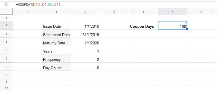
As you can see, settlement date, maturity date, frequency, and day count are the required arguments that are highlighted.
Formula:
=COUPDAYS(C3,C4,C6,C7)The COUPDAYS formula in cell F2 returns the number of coupon days as 180. Change the frequency in cell C6 to 1. The formula will then return 360 days.
That means frequency 1 = 360 days, 2 = 180 days, and 4 = 90 days. If you change the day count from 0 to 1, the result will be 365 days, 181 days, and 90 days respectively.
In concise the day count convention indicator plays an important role in the coupon days calculation using COUPDAYS Function in Google Sheets.
Input Values (COUPDAYS Arguments) within Formula
When you directly use the input values within the COUPDAYS function in Google Sheets, use the DATE function to input settlement and maturity dates.
For example, the settlement date 31/1/2019 and maturity date 1/1/2020 must be entered as date(2019,1,31) and date(2020,1,1) respectively.
Even if your settlement and maturity dates are in mm/dd/yyyy format, you must use the DATE formula as above.
Common Errors in COUPDAYS Function Use in Google Sheets
There are two common errors Google Sheets may return when using COUPDAYS function in Google Sheets. They are #VALUE! and #NUM!
Reasons
Invalid input of dates causes the #VALUE! error.
If frequency, as well as the day count indicators, are not the specified values (out of range), COUPDAYS will return the #NUM! error value.
One more reason for the #NUM! error is settlement ≥ maturity.
That’s all. Enjoy!