Google Sheets has no specific function to count the number of cells in a range directly. However, you can achieve this by using certain function combinations. There are two main options: multiplying the number of rows and columns in the range, or conditionally counting the cells. We will explore both options.
Count the Number of Cells Using ROWS and COLUMNS Functions
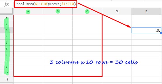
Let’s say you want to find how many cells are in the range A1:C10.
You can use one of the following formulas:
=ROWS(A1:C10)*COLUMNS(A1:C10)or
=SUMPRODUCT(ROWS(A1:C10), COLUMNS(A1:C10))In these formulas:
- The ROWS function returns the number of rows in the range.
- The COLUMNS function returns the number of columns in the range.
By multiplying the two, you get the total number of cells in the specified range.

Count the Number of Cells Using the COUNTIF Function
Another method to count the number of cells in a range is by using the COUNTIF function.
=ARRAYFORMULA(COUNTIF(A1:C10&"", "*"))In this formula:
- We concatenate an empty string (
&"") to the rangeA1:C10to ensure it is considered non-blank. This allows the COUNTIF function to count the cells in the range. - The asterisk (
*) is a wildcard that represents any number of characters (including none), which makes it useful for counting all cells.
This formula will return the total number of cells in the range that are non-blank.
Real-Life Use
You can use the formula above to check if all cells in the range are filled or not.
For example, to check if all cells in the range A1:C10 are non-empty, use the following formula:
=COUNTA(A1:C10)=ROWS(A1:C10)*COLUMNS(A1:C10)This will return TRUE if all cells are filled and FALSE if any cell is empty.
- The first part,
COUNTA(A1:C10), counts the number of non-empty cells. - The second part,
ROWS(A1:C10) * COLUMNS(A1:C10), gives the total number of cells in the range.
You can also modify this formula to check for specific values. For example, to check if all cells in the range A1:C10 contain the word “Apple,” use:
=COUNTIF(A1:C10, "Apple")=ROWS(A1:C10)*COLUMNS(A1:C10)This will return TRUE if every cell in the range contains “Apple.”
Conditional Formatting
If you want to apply conditional formatting based on the above evaluations, remember to use absolute references for the range.
For example, to highlight any cell (e.g., D1) if all cells in A1:C10 contain “Apple,” use the following formula:
=COUNTIF($A$1:$C$10, "Apple")=ROWS($A$1:$C$10)*COLUMNS($A$1:$C$10)To apply the rule:
- Navigate to cell
D1. - Click
Format>Conditional formatting. - Select Custom formula is under Format Rules, and enter the above formula.


