Google Sheets has recently introduced several features, with one of the latest being the ability to insert tables. You can now insert custom tables and also convert a range to a table in Google Sheets. This tutorial will guide you through the process of converting a range to a table and vice versa.

Until now, we’ve been relying on a workaround (you can find it here: How to Create Self-Formatting Tables in Google Sheets (With a Simple Initial Setup)), which has several limitations. However, we no longer depend on such workarounds.

Before you begin, ensure that your data meets the following three basic requirements to convert a table to a range in Google Sheets:

1. There should not be any formulas in the top row of the range.
2. If there isn’t a header row with field labels, insert a blank row at the top of the range.
3. There should not be merged cells in the range.

Once you meet these requirements, you can proceed to convert a range to a table in Google Sheets.

Converting a Range to a Table in Google Sheets

Example #1: Range with Header Row

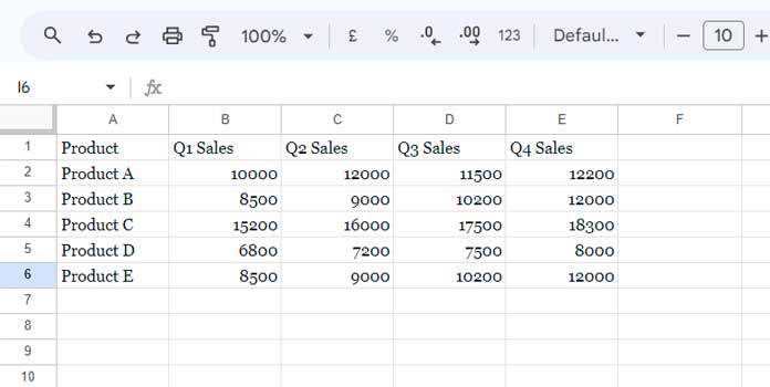
I have the following sample data in the range A1:E6 where A1:E1 contains the field labels “Product”, “Q1 Sales”, “Q2 Sales”, “Q3 Sales”, and “Q4 Sales”.

Here are the step-by-step instructions to convert this range to a table:

1. Select the range A1:E6.
2. To open the context menu, right-click any cell within the selected range.
3. Select “Convert to table”.

It’s as simple as that.

Example #2: Range without a Header Row

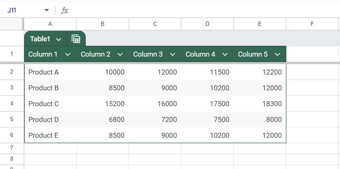
Let’s consider the same sample data as above but without the header row. In other words, the data is in A2:E6, and A1:E1 is empty.

You can follow the same steps as above: select A1:E6, then right-click any cell within the selected range, and choose “Convert to table”.

Google Sheets will add field labels in the top row like “Column 1”, “Column 2”, … “Column 5”.

Converting a Table to a Range in Google Sheets

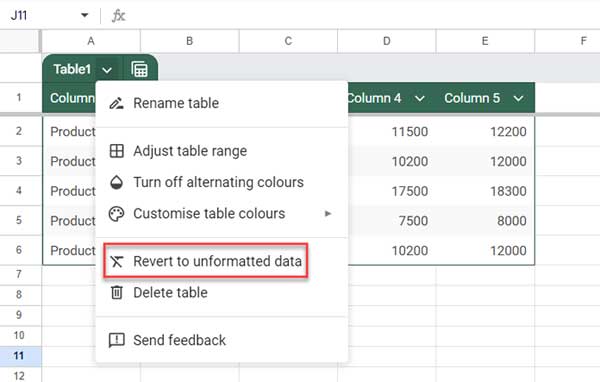
To convert a table back to a range, follow these steps:

1. Open the “Table menu” by clicking on the dropdown next to the table name at the top left corner of the table.
2. Then select “Revert to unformatted data”.

Optionally, Go to the View menu and click on Freeze > No rows.

Conclusion

Unlike a data range, a table offers several advantages, particularly in data formatting. You can assign data types to columns by clicking the dropdown in the header of each column and selecting “Edit column type”. This feature is very useful when multiple users update the table with content, as it helps avoid mixed data type issues in columns.

Another notable feature is the use of table names in formulas. So, when the table grows, the formula will automatically adjust to use the correct range.

Example formulas:

=SUM(Table1[Q1 Sales])

Where ‘Table1’ represents the table name and ‘Q1 Sales’ represents the field label of the second column (as per example #1).

=QUERY(Table1[#ALL], "Select A, sum(C) group by A")

Where ‘Table1’ represents the table name and #ALL represents all fields in the table (as per example #1).

I hope you enjoy using this new Google Sheets feature and find it helpful when converting your ranges to tables and vice versa in Google Sheets.

Resources

• Structured Table References in Formulas in Google Sheets
• Customizing Alternating Colors of a Table in Google Sheets