Common Errors in VLOOKUP in Google Sheets

Whether you’re just getting started or have used VLOOKUP hundreds of times, chances are you’ve run into a few frustrating errors. Don’t worry — you’re not alone. In this guide, I’ll walk you through the most common errors in VLOOKUP in Google Sheets, why they happen, and how to fix them quickly.

To keep things simple, I’ve grouped these into two main types:

Syntax errors — These trigger actual error messages like #N/A!, #REF!, #VALUE!, #ERROR!, and #NAME?.
Accidental mistakes — These won’t trigger an error message but might give you the wrong result, which is arguably worse.

Let’s tackle each one — with clear examples and fixes.

Syntax-Based Errors in VLOOKUP

These are the typical VLOOKUP errors that throw up #N/A, #REF!, #VALUE!, and other error messages when your formula syntax goes wrong.

1. #N/A! — Not Found Error

Tooltip: Did not find value ‘Student 6’ in VLOOKUP evaluation.

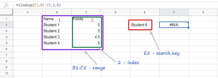
This is hands down the most common error in VLOOKUP. It simply means: “I looked, but I didn’t find what you asked for.”

Example:

=VLOOKUP(E2, B1:C5, 2, FALSE)

If the value in E2 (“Student 6”) isn’t in the first column of the range (B1:B5), VLOOKUP gives you the dreaded #N/A!.

How to Fix or Hide the #N/A!

You’ve got a few options depending on what you want to show instead of the error:

Return a blank:
=IFNA(VLOOKUP(E2, B1:C5, 2, FALSE))
Return a custom message:
=IFNA(VLOOKUP(E2, B1:C5, 2, FALSE), "Student not found")
Return 0 instead:
=IFNA(VLOOKUP(E2, B1:C5, 2, FALSE), 0)

A Note on IFERROR vs. IFNA

Yes, you could also use IFERROR, but here’s the thing: it’ll catch any error, not just #N/A!. That might hide more than you’d like — including real issues with your formula. So when you’re specifically handling #N/A!, stick with IFNA.

2. #VALUE! — Argument Error

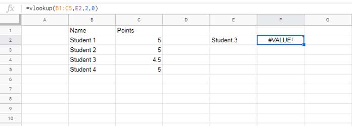
The #VALUE! error usually means there’s a problem with how you’ve entered the arguments in your VLOOKUP formula.

Common #VALUE! error in VLOOKUP in Google Sheets

Common Scenarios:

Wrong order of arguments:
=VLOOKUP(B1:C5, E2, 2, FALSE)
❌ Here, you’re putting the range first and the search key second — that won’t work.
✅ Correct it like this:
=VLOOKUP(E2, B1:C5, 2, FALSE)
Using text instead of a column number:
=VLOOKUP(E2, B1:C5, "Points", FALSE)
The third argument (column index) should be a number — not a label. So use 2 instead of "Points".
Index is 0 (or less than 1):
=VLOOKUP(E2, B1:C5, 0, FALSE)
VLOOKUP columns start from 1, not 0 — so using 0 triggers this error.

3. #REF! — Invalid Reference

You’ll see #REF! when VLOOKUP points to a range that no longer exists.

Example:

=VLOOKUP(C2, #REF!, 2, FALSE)

Maybe you deleted the original range, or the formula refers to cells that never existed — like using an invalid sheet name in the range (e.g., Sales!A1:C when the actual sheet is named SalesData).

Out-of-Bounds Range Example:

=VLOOKUP(E2, B1001:C10000, 2, FALSE)

If your sheet only has 1,000 rows, and you’re referencing from row 1001 onwards — well, that’s going to break the formula.

You’ll see a similar error if your index number is out of bounds — for example, if your range only has 2 columns but you enter 3 as the index. VLOOKUP can’t return a column that doesn’t exist in the range.

4. #ERROR! — Formula Parse Errors

This error usually pops up when there’s something Google Sheets can’t interpret — like missing quotes, invalid references, or broken syntax.

Common Scenarios:

Unquoted sheet name with spaces:

=VLOOKUP("Apple", Sales Report!A1:B, 2, FALSE)

❌ This causes a formula parse error.
✅ Fix it by adding single quotes:

=VLOOKUP("Apple", 'Sales Report'!A1:B, 2, FALSE)

Invalid structured table reference:

=VLOOKUP("Ben", Table2[#ALL], 2, FALSE)

If Table2 doesn’t exist (or isn’t created via Insert > Table), this will break with an error.

5. #NAME? — Typo or Undefined Name

This error often pops up because of:

A typo in the function name:
=vlokup(E2, B1:C5, 2, FALSE) ← typo!
Using a named range that doesn’t exist:
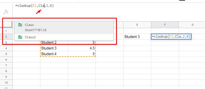
=VLOOKUP(E2, Classs, 2, FALSE)
Using a field label like “Points” instead of a column index:
=VLOOKUP(E2, B1:C5, Points, FALSE) (Only database functions like DGET allow field labels — VLOOKUP doesn’t.)

Pro Tip:

If you’re using Named Ranges, Google Sheets will auto-suggest them as you type. Just pick from the dropdown — that way, no spelling errors.

Accidental Mistakes That Break VLOOKUP

Now for the sneaky stuff — when your formula doesn’t throw an error but still gives you the wrong result.

1. Extra Spaces

Spaces at the start or end of a value are invisible — but deadly in lookups.

Example:

Even this tiny space causes a mismatch:

=VLOOKUP("Student 3 ", B1:C5, 2, FALSE)

In this case, there’s an accidental space after “Student 3” — and VLOOKUP won’t find a match.

Fix:

Make sure the search_key doesn’t include any extra spaces. A simple typo like that can return #N/A.

You can clean up your data in two ways:

Manual option:
Select the column → go to Data → Data clean-up → Trim whitespace
Formula-based fix:
Use TRIM() inside VLOOKUP to clean the lookup range:
=ARRAYFORMULA(VLOOKUP(E2, TRIM(B1:C5), 2, FALSE))

And if the issue is on the search_key side (like in "Student 3 "), you can also wrap that with TRIM():

=VLOOKUP(TRIM(E2), B1:C5, 2, FALSE)

2. Format Mismatch (Text vs. Number vs. Date)

If your search key is a number but the column is formatted as text, VLOOKUP might return #N/A! — even if the numbers look the same.

Example Fixes:

Ensure the first column in your range is formatted as Number, not Text.
For dates, both your search key and range must use the same format (e.g., DD/MM/YYYY).

3. Wrong Match Type (is_sorted Argument)

This is a big one.

If you forget to specify the fourth argument in VLOOKUP (is_sorted), Google Sheets assumes it’s TRUE — which means “approximate match”.

Result:

You might get a wrong result that looks right — and never realize it.

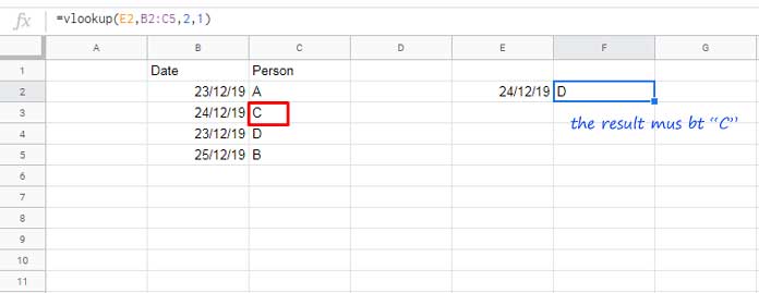
Best Practice:

Unless you know what you’re doing, always set it to FALSE:

=VLOOKUP(E2, B2:C5, 2, FALSE)

Or, if your data isn’t sorted and you do want an approximate match, sort it within the formula using SORT():

=VLOOKUP(E2, SORT(B2:C5, 1, TRUE), 2, TRUE)

Conclusion

That wraps up the most common errors in VLOOKUP in Google Sheets — both the ones that throw errors and the ones that sneak past without you noticing.

Get these right, and your formulas will become far more reliable (and less stressful to debug!).

More VLOOKUP Guides and Use Cases in Google Sheets

Looking to explore more? Here are some in-depth tutorials to level up your VLOOKUP skills in Google Sheets.