The color scale in Google Sheets’ conditional formatting helps us to apply gradient colors to a range based on lower and upper values.
For example, if you have a range containing students’ marks, you can highlight it with one click, where higher values get dark shades of Red and lower values get light shades of Red.
You can apply light to dark or vice versa based on your choice. It only applies to numbers, dates, and timestamps in a range.
If you have numbers mixed with text in a cell, you should extract that number before formatting.
For that, you can depend on functions like Regexextract and Regexreplace.
Four color scale formatting rules/options are available in Google Sheets under the Format menu Conditional formatting.
- Min and Max.
- Number.
- Percentile.
- Percent.
Let’s see how to use these color scale format rules in Conditional formatting in Google Sheets.
1. Min and Max Color Scale in Google Sheets
In this color scale formatting, you won’t be able to specify the min and max values.
The Sheet, I mean the command, will automatically pick it from the range.
Select B3:B14 and go to the menu Format > Conditional formatting > Color scale and follow the below settings.
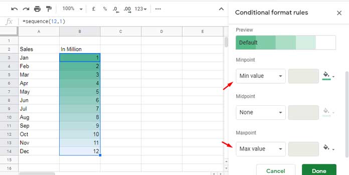
By default, the min value in the range has the darkest color Green, and the max value has the brightest color, White. That means Green to White.
Don’t like this? You can choose from the preset or create a custom color scale under “Preview.”
2. Number Color Scale in Google Sheets
Assume you want the gradient colors applied to numbers between 3.75 and 9.25, both inclusive, in a range.
In that case, you can use the number color scale in Google Sheets.
Specify Minpoint as 3.75 and Maxpoint as 9.25 and see the result.
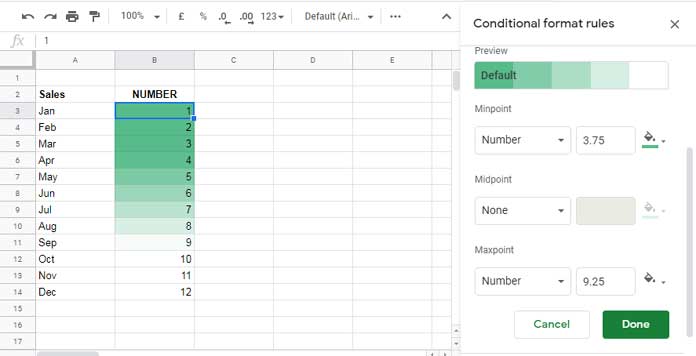
What about the numbers that fall outside of this range?
In my example, the min has a darker shade of Green. So the values below the min value will inherit the same color.
Since the max value has a White color scale applied, the values above the max will have the same color.
Tip:- You can opt for the mix of Min-Max (1) or Number (2) color scale in Google Sheets.
3. Percentile Color Scale in Google Sheets
I have used the min and max numbers 3.75 and 9.25 in the above example with a purpose. We will use that with the Percentile color scale example below.
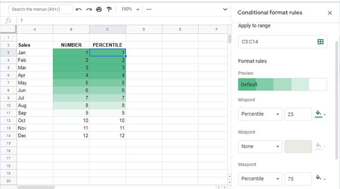
The min number 3.75 is closest to the 25% mark, and the max number 9.25 is closest to the 75% mark in the range B3:B14.
If you want, you can test that using the below Percentile formulas in your Sheet.
25% Mark:
=percentile(B3:B14,0.25)75% Mark:
=percentile(B3:B14,0.75)For testing, you can use the equivalent Quartile formulas also.
1st Quartile (25% mark):
=QUARTILE(B3:B14,1)3rd Quartile (75% mark):
=QUARTILE(B3:B14,3)Set Minpoit to 25 and Maxpoint to 75 in the Percentile color scale in Google Sheets.
It will match the same number formatting with the values 3.25 (min) and 9.25 (max).
Here in the Percentile color scale, the advantage is, Sheets automatically calculates the min and max points based on the given percentile.
3. Percent Color Scale in Google Sheets
It’s different from the above two (Number and Percentile).
Let me adjust the data, then apply the conditional formatting. If you use the above same data, you won’t be able to see the difference.
Here let’s use the Midpoint also. The color scheme used is Green (Min) – Red (Mid) – White (Max).
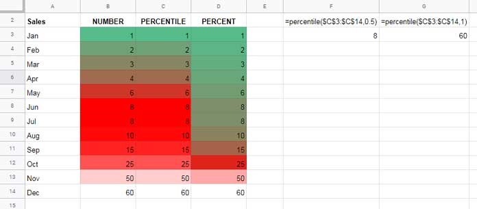
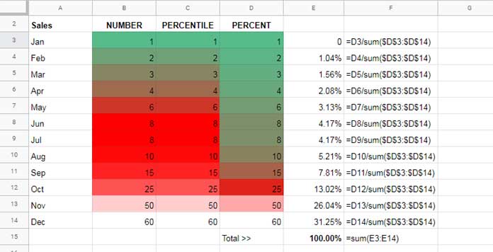
Range B3:B14 (Number): Minpoint # 1, Midpoint # 8, and Maxpoint 60.
Range C3:C14 (Percentile): Minpoint # 0, Midpoint # 50, and Maxpoint 100.
If you check the image, you can see columns B and C have the same gradient colors.
It is because the 0, 50, and 100 percentiles are equal to the numbers 1, 8, and 60, respectively.
Tip:- If you update values in B3:B14, the Min, Mid, and Maxpoint values won’t update within the Conditional format rules panel. I have a workaround in a later part below.
Range D3:D14 (Percent): Minpoint # 0, Midpoint # 50, and Maxpoint 100.
Percent color grading in column D is different in comparison to the Percentile color grading in column C.
It’s because the Percent conditional format is based on the percent distribution of the range of values present.
Using Cell References in Minpoint, Midpoint, and Maxpoint
Can we use a cell value instead of hand enter them within the color scale panel in Google Sheets?
Yes! You usually find it useful with the Number color scale, even though the other two, i.e., the Percentile, and Percent, support it.
For example, enter 3.75 in cell F1 and 9.25 in cell F2. You can specify them (point to those cells) within the Conditional formatting panel as below.
Enter =$F$1 instead of 3.25 in Minpoint and =$F$2 instead of 9.25 in Maxpoint.
That’s all, enjoy!


