The CEILING function in Google Sheets allows you to round a number up to the nearest integer multiple of a specified significance. In contrast, the FLOOR function rounds a number down, while the MROUND function rounds a number to the nearest integer multiple of another number. Understanding these functions can simplify your calculations and data manipulation in Google Sheets.

Syntax

CEILING(value, [factor])

Arguments

• value: The number you want to round up.
• factor (optional): The multiple to which you want to round the value. If omitted, it defaults to 1. Note that the factor cannot be 0 and must be positive.

Example of the CEILING Function in Google Sheets

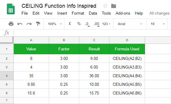
Let’s explore how to use the CEILING function with a few examples. Note that the formula results (Column C) will always be greater than or equal to the values in Column A.

Example Formula

Using direct values instead of cell references, you can write:

=CEILING(8, 3)

Result: 9

In this formula, 8 is the value and 3 is the factor. The CEILING function rounds 8 up to the nearest integer multiple of 3.

If you were to use the FLOOR function in this case:

=FLOOR(8, 3)

Result: 6

Here, the FLOOR function rounds 8 down to the nearest multiple of 3. The multiples of 3 are:

• 1 x 3 =3
• 2 x 3= 6
• 3 x 3 = 9

Since 8 is closer to 9 when rounding up, the CEILING function returns 9.

Important Notes

1. The factor argument is optional, but if you omit it, the function treats it as 1.
2. The factor must be positive; the value can be either positive or negative.
3. CEILING is commonly used to round up decimal values. For example:

=CEILING(23.91, 0.05)

Result: 23.95

Practical Use Case: Currency Conversion

You can utilize the CEILING function in Google Sheets to round up currency denominations. For example, at the time of writing, the exchange rate from INR to USD is approximately 0.01189029, meaning 1 INR equals 0.01189029 USD. (I obtained this value using the GOOGLEFINANCE function, such as =GOOGLEFINANCE("CURRENCY:INRUSD").) Therefore, converting 1450.00 INR to USD gives you:

=1450 * 0.01189029

This equals approximately 17.2269205 USD. To round this amount up to the nearest 5 cents, use the CEILING function:

=CEILING(17.2269205, 0.05)

Result: 17.25 USD

This helps ensure you’re always rounding up to a more convenient currency value.

Conclusion

The CEILING function is a powerful tool for rounding numbers up to specific increments in Google Sheets. Understanding its syntax and how it compares with similar functions like FLOOR and MROUND will enhance your data manipulation skills.

Enjoy using the CEILING function in your spreadsheets!