


")


")

")
")
 in Excel & Google Sheets")


A calendar heatmap visualizes the magnitude of daily values within a month using color intensity. The underlying dataset can be anything recorded on a daily basis—such as sales amounts, quantities sold, expenses, or activity counts.
You can enter these values directly into the calendar grid or populate them dynamically using formulas. For example, XLOOKUP works well when there is only one transaction per day, while SUMIF or COUNTIF is more suitable when multiple entries exist for the same date.
Google Sheets does not offer a built-in calendar heatmap. The native heatmap (color scale) cannot be applied directly to a calendar layout because dates are stored internally as serial numbers. This causes conflicts between the date grid and the value-based color scale.
To overcome this, this Calendar Heatmap Template in Google Sheets uses conditional formatting with custom colors—but in a novel way. Instead of relying on up to 31 automatic shades, the values are grouped into 7 well-defined buckets. The scale is split at 0, with separate buckets for positive and negative values. As a result, the calendar heatmap becomes two-sided, clearly highlighting both gains and losses when negative values are present.

Before we go into how to use the calendar heatmap, you can get the template by clicking the button below:
How to Use the Calendar Heatmap Template in Google Sheets
Using this Calendar Heatmap Template in Google Sheets is straightforward. However, the approach depends on whether you:
- Enter data manually within the calendar grid, or
- Fetch data dynamically from another sheet (for example, a sales table).
Let’s start with manual data entry.
Manual Data Entry in the Calendar Heatmap
1. Set Up the Control Panel
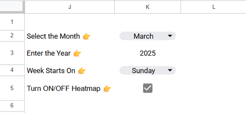
The calendar heatmap includes a control panel located at the top-right of the calendar grid with the following options:
- Select the Month
- Enter the Year
- Week Starts On
- Turn ON/OFF Heatmap
Select the Month and Year
First, select the month (cell K2) and enter the year (cell K3) for which you want to record data. The calendar grid will automatically populate with the corresponding dates.
Week Starts On
By default, the calendar displays weeks from Sunday to Saturday. If you prefer a Monday–Sunday layout, select Monday from cell K4.
Turn ON/OFF Heatmap
The checkbox in cell K5 allows you to toggle the heatmap on or off. This is useful when you want to print the calendar or view it without color formatting.
2. Understanding the Calendar Layout
Once the control panel settings are selected:
- The top row (Row 1) displays the header automatically in the format MMMM YYYY.
- Dates belonging to the selected month and year appear within the calendar grid, displayed as DD and left-aligned.
- Below each week row, there is an extra row for entering data.
These data-entry rows are: Rows 5, 7, 9, 11, 13, and 15.
3. Enter Your Daily Data Manually
Enter each day’s value in rows 5, 7, 9, 11, 13, and 15, directly under the corresponding date.
Once entered, the heatmap colors update automatically.
4. Adding Data for Another Month
After filling in a calendar, do not change the existing control panel settings, except for the Heatmap ON/OFF toggle. If you change the month, year, or week start setting, the calendar layout will update, but the data you manually entered will no longer be valid because it belongs to a different month.
So, what should you do if you want to enter data for another month?
The solution is to keep the current calendar as is and make a copy of it.
To create a calendar for another month:
- Click the drop-down arrow next to the sheet tab.
- Select Duplicate.
- In the duplicated sheet, choose a new month (and year, if required) in the control panel.
- Clear the existing values in the calendar grid.
- Enter the new month’s data.
This approach allows you to maintain one calendar sheet per month while preserving previously entered data.
Lookup Data from Another Tab in the Calendar Heatmap
This is the dynamic way to use the Calendar Heatmap Template in Google Sheets. Instead of duplicating the calendar for each month, you use a single calendar that pulls data from a separate table.
The formula depends on whether you have:
- One transaction per day, or
- Multiple transactions per day.
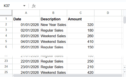
1. When You Have One Transaction per Day
- Click Insert > Sheet from the menu to add a new sheet.
- Right-click the sheet tab, choose Rename, enter Data, and press Enter.
- In row 1, enter the following headers:
- A1: Date
- B1: Description
- C1: Amount / Quantity
- Enter:
- Dates (no timestamps) in A2:A
- Descriptions in B2:B
- Values in C2:C
- Go back to the heatmap sheet.
- Before entering the formula, clear any manually entered data in the calendar grid to avoid conflicts.
Then enter the following formula in cell B5:
=ArrayFormula(XLOOKUP(B4:H4, Data!$A:$A, Data!$C:$C,))- Copy the formula from B5 and paste it into:
- B7, B9, B11, B13, and B15
You can now change the month and year in the control panel to view data dynamically within the calendar. This is the recommended way to use the calendar heatmap.
2. When You Have Multiple Transactions per Day
Replace the previous formula with one of the following, depending on your requirement.
To calculate totals:
=ArrayFormula(IF(B4:H4, SUMIF(Data!$A:$A, B4:H4, Data!$C:$C),))To calculate counts:
=ArrayFormula(IF(B4:H4, COUNTIF(Data!$A:$A, B4:H4),))Enter the formula in B5 and copy it to every alternate data row, as explained earlier.
Conclusion
In this guide, we explored how to use a Calendar Heatmap Template in Google Sheets—both with manual entry and dynamic lookup methods. If you’re interested in building the template yourself, you can follow the step-by-step guide linked below.