Calculate Trip Days by Month (Start, End, and Full Days) in Google Sheets

If you’re managing business travel in Google Sheets, you may need to calculate how many full days a trip spans in each calendar month—especially when companies provide food allowances only for full days, excluding the trip start and end dates. In many cases, these allowances are processed monthly, so breaking down the trip duration by month becomes essential.

Unfortunately, there’s no built-in function in Google Sheets to calculate trip days by month, including separate counts for full days and start/end days. But with a smart combination of formulas, you can dynamically calculate trip duration by month in Google Sheets—even when the trip spans multiple months.

In this tutorial, I’ll show you how to build a formula that splits trip days by month and identifies the start, end, and full days. Whether you’re handling employee reimbursements or managing travel logs, this method will save you time and improve accuracy.

Note:

I’ve created two formulas:

If you just want to calculate the trip duration by month from a single start and end date, use the formula in Example 1.
If you have a list of start and end dates, use the formula in Example 2.

Both formulas follow the same logic. However, the second one uses a LAMBDA with MAP to iterate over rows, so it’s more resource-intensive. If you’re working with just one trip, stick to the first formula to avoid unnecessary load.

Example 1: Calculate Trip Days Duration by Month from a Single Start and End Date

Assume the trip start date is in cell A2 and the end date in B2.

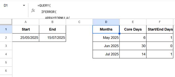
Google Sheets formula calculating trip days by month from start and end date

Use this formula in cell D1:

=QUERY(
  IFERROR(
    ARRAYFORMULA(
      LET(
        start, INT(A2), 
        end, INT(B2) , 
        full_months, EDATE(EOMONTH(start, -1)+1, SEQUENCE(DATEDIF(start, end, "M"))), 
        boundary_dates_list, UNIQUE(TOCOL(VSTACK(start, full_months, IF(EOMONTH(start, 0)=EOMONTH(end, 0),, EOMONTH(end, -1)+1), end), 3)), 
        data, HSTACK(EOMONTH(boundary_dates_list, -1)+1, CHOOSEROWS(boundary_dates_list, SEQUENCE(ROWS(boundary_dates_list)-1, 1, 2))-boundary_dates_list-VSTACK(1, SEQUENCE(ROWS(boundary_dates_list)-1, 1, 0, 0)), VSTACK(1, TOCOL(SEQUENCE(ROWS(boundary_dates_list)-2, 1, 0, 0), 3), 1)), data
      )
    )
  ), "select Col1, sum(Col2), sum(Col3) where Col1 is not null group by Col1 label Col1 'Months', sum(Col2) 'Core Days', sum(Col3) ' Start/End Days' format Col1 'MMM YYYY'", 0
  )

⚠️ Important Note: If the start and end dates are the same, this formula will return an error. It only works when there is at least one full day between them.

How the Formula Works (Optional)

If you’re already familiar with functions like QUERY, SEQUENCE, EDATE, and DATEDIF, this breakdown will help you understand how the formula calculates trip duration by month in Google Sheets.

We used LET to define reusable variables:

1. `start` and `end`:

start, INT(A2)
end, INT(B2)

These remove the time components, if present, from the dates.

2. `full_months`:

EDATE(EOMONTH(start, -1)+1, SEQUENCE(DATEDIF(start, end, "M")))

DATEDIF(start, end, "M") gives the number of full months.
EDATE returns the first date of each full month in the trip.
If a trip spans from May 25 to July 15, this gives you June 1.

3. `boundary_dates_list`:

UNIQUE(TOCOL(VSTACK(start, full_months, IF(EOMONTH(start, 0)=EOMONTH(end, 0),, EOMONTH(end, -1)+1), end), 3))

This part is the heart of calculating the trip duration by month. Here’s what it does:

It creates a column of boundary dates, including:

the trip start date,
the first day of any full months between the start and end dates (if the trip spans more than one month),
and the trip end date.

For example, if the trip starts on May 25 and ends on July 15, the boundary dates would be:

We generate this list by stacking the start and end dates along with full_months. However, full_months may return an error in two cases:

if the start and end dates fall in the same month,
or if they span across two different months but not full months in between.

In the first case, the error is acceptable. But in the second, we still need to include the start of the last month, which EOMONTH(end, -1) + 1 provides. The formula adds this conditionally.

Since this stacking may create duplicate dates, we wrap the result with UNIQUE to remove them. TOCOL flattens the list into a single column and also filters out any errors.

This results in a clean list of date boundaries. Subtracting each date from the next in this list will give us the number of trip days that fall within each month. That’s exactly what the next step does.

4. `data`:

HSTACK(
   EOMONTH(boundary_dates_list, -1)+1, 
   CHOOSEROWS(boundary_dates_list, SEQUENCE(ROWS(boundary_dates_list)-1, 1, 2))-boundary_dates_list-VSTACK(1, SEQUENCE(ROWS(boundary_dates_list)-1, 1, 0, 0)), 
   VSTACK(1, TOCOL(SEQUENCE(ROWS(boundary_dates_list)-2, 1, 0, 0), 3), 1)
)

This section prepares the dataset for the final QUERY step as follows:

Column 1	Column 2	Column 3
01/05/2025	6	1
01/06/2025	30	0
01/07/2025	14	0
01/07/2025	#N/A	1

Here’s how it works:

First column:
EOMONTH(boundary_dates_list, -1) + 1 returns the start of the month for each segment. This is used as the grouping label for monthly summaries.
Second column:
Calculates the number of days between each boundary date and the one that follows.
Then we subtract 1 from only the first row to exclude the trip start date.
The trip end date is excluded automatically because it doesn’t have a following date, so the subtraction results in #N/A. For example (as per the boundary_dates_list above):
- Segment 1: May 25 to June 1 → 7 - 1 = 6 full days
- Segment 2: June 1 to July 1 → 30 full days
- Segment 3: July 1 to June 15 → 14 full days
- Segment 4: End date only → #N/A (no subtraction)
Third column:
Marks start and end segments with 1, and everything else with 0.
This allows the final QUERY to separately count the core (full) days and start/end days for each month.

Example 2: Calculate Trip Days Duration by Month from a List of Start and End Dates

If your trip data spans multiple rows (e.g., column A for start dates, column B for end dates), use this version:

=QUERY(
   IFERROR(WRAPROWS(TOROW(
      LET(
         table, FILTER(A2:B, LEN(A2:A)), 
         MAP(CHOOSECOLS(table, 1), CHOOSECOLS(table, 2), LAMBDA(_start, _end, TOROW(
            ARRAYFORMULA(LET(
               start, INT(_start), 
               end, INT(_end), 
               full_months, EDATE(EOMONTH(start, -1)+1, SEQUENCE(DATEDIF(start, end, "M"))), 
               boundary_dates_list, UNIQUE(TOCOL(VSTACK(start, full_months, IF(EOMONTH(start, 0)=EOMONTH(end, 0),, EOMONTH(end, -1)+1), end), 3)),
               data, HSTACK(EOMONTH(boundary_dates_list, -1)+1, CHOOSEROWS(boundary_dates_list, SEQUENCE(ROWS(boundary_dates_list)-1, 1, 2))-boundary_dates_list-VSTACK(1, SEQUENCE(ROWS(boundary_dates_list)-1, 1, 0, 0)), VSTACK(1, TOCOL(SEQUENCE(ROWS(boundary_dates_list)-2, 1, 0, 0), 3), 1)), 
               data
            ))
         )))
      )), 3)
   ), "select Col1, sum(Col2), sum(Col3) where Col1 is not null group by Col1 label Col1 'Months', sum(Col2) 'Core Days', sum(Col3) ' Start/End Days' format Col1 'MMM YYYY'", 0
)

Replace A2:B with the full date range, and A2:A with just the start date column.

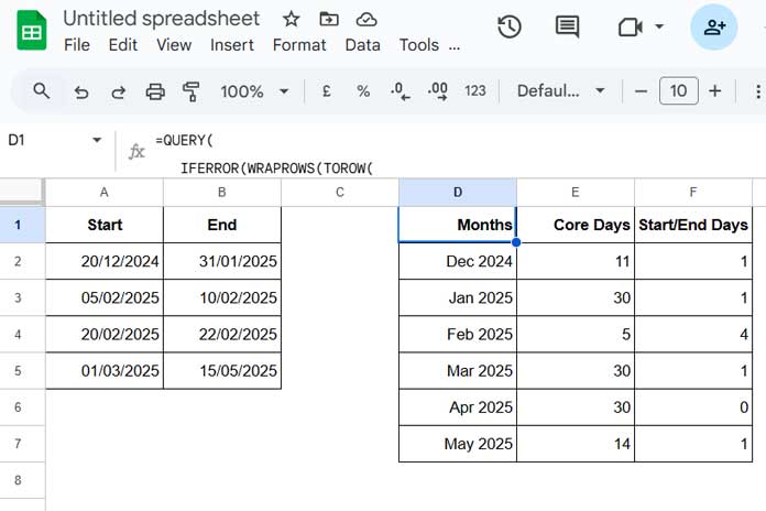
Calculating trip duration by month from a list of start and end dates in Google Sheets

This will return the trip duration by month for the entire list of date ranges in one go.

The formula uses the same core logic as the earlier example to calculate trip days by month in Google Sheets, but with one key difference: before feeding the result (data) into the QUERY function, we first transform the data from each row into a single row using TOROW. This allows us to loop through each row using MAP, process each trip’s data individually, and then stack all the results into one continuous row. Finally, we reshape that long row into 3 columns and summarize it using QUERY.

Conclusion

Using these formulas, you can calculate trip duration by month in Google Sheets while clearly separating full days from start and end dates. This is especially useful in real-world scenarios like travel reimbursements, per diem tracking, or monthly reporting.