How to Find the Bottom-Right Corner of Your Data in Google Sheets

In several cases, you may need to find the bottom-right corner of your data in Google Sheets. This is especially useful when creating dynamic ranges because it lets you restrict formulas to just the active portion of your dataset instead of entire open ranges like A1:1000 or A1:Z.

The bottom-right corner is defined as the cell where the lowest filled row in the dataset meets the rightmost filled column. For example, if your dataset covers A1:Z50 but the last filled row is row 10 and the last filled column is column K, then the bottom-right corner is K10. The effective used range would then be A1:K10.

Important: Place the formulas outside the dataset (or on another sheet) to avoid circular reference errors.

Table of Contents

Why You May Need to Find the Bottom-Right Corner in Google Sheets

To build INDIRECT ranges that don’t expand unnecessarily.
To handle datasets that grow both downwards and across columns.

When working with a single column or row, finding the last filled cell is straightforward. One way to do this is:

=ArrayFormula(XMATCH(TRUE, A1:A<>"", 0, -1))  // last row in column A
=ArrayFormula(XMATCH(TRUE, A1:1<>"", 0, -1))  // last column in row 1

For multi-row, multi-column ranges, the bottom-right corner is the cell where the lowest filled row meets the rightmost filled column.

Animated Google Sheets example showing the bottom-right corner cell updating dynamically as new values are entered

Find the Address of the Last Used Cell Intersection in Google Sheets

Here are two formulas you can use to dynamically find the bottom-right corner.

Using a LAMBDA Formula to Find the Bottom-Right Corner

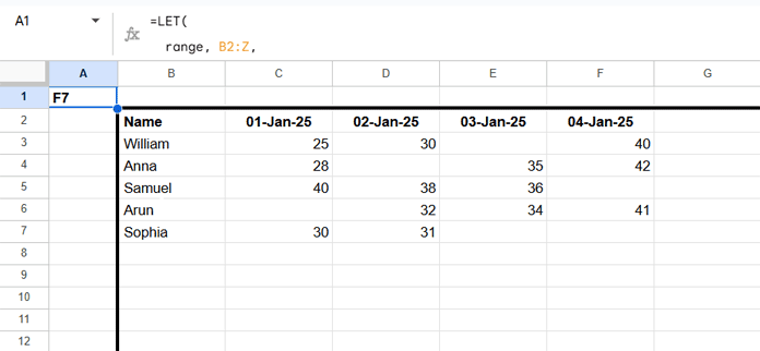
Suppose your dataset is in B2:Z.

To get the bottom-right corner, enter this formula outside the dataset:

=LET(
  range, B2:Z, 
  start, ADDRESS(MIN(ROW(range)), MIN(COLUMN(range)), 4), 
  colL, REGEXEXTRACT(
    ADDRESS(1, 
      MAX(BYCOL(range, LAMBDA(val, IF(COUNTA(val), COLUMN(val)))))),
    "[A-Z]+"
  ), 
  rowN, MAX(BYROW(range, LAMBDA(val, IF(COUNTA(val), ROW(val))))), 
  JOIN(, colL, rowN)
)

✅ Output: F7 (the bottom-right corner of the dataset).

Google Sheets formula output showing F7 as the bottom-right corner of the dataset

Find the Actual Used Range

If you want the full used range (e.g., B2:F7), replace:

JOIN(, colL, rowN)

with:

JOIN(, start, ":", colL, rowN)

Google Sheets formula output showing the full used range B2:F7 instead of only the bottom-right cell

Formula Explanation

ADDRESS(MIN(ROW(range)), MIN(COLUMN(range)), 4) → returns the top-left corner of the range.
BYCOL(range, LAMBDA(val, IF(COUNTA(val), COLUMN(val)))) → checks each column for non-empty cells and returns its column number if it contains data.
MAX(...) → picks the rightmost column with data.
REGEXEXTRACT(ADDRESS(1, ...), "[A-Z]+") → converts the column number to a column letter.
BYROW(range, LAMBDA(val, IF(COUNTA(val), ROW(val)))) → returns row numbers of non-empty rows.
MAX(...) → picks the lowest filled row.
JOIN(, colL, rowN) → combines the rightmost column and lowest row into the bottom-right cell address.
JOIN(, start, ":", colL, rowN) → combines the top-left and bottom-right corners to return the full used range.

Find the Bottom-Right Corner Without LAMBDA (Best for Large Data)

If the LAMBDA version slows down with large datasets, use this formula:

=ArrayFormula(LET(
  range, B2:Z, 
  start, ADDRESS(MIN(ROW(range)), MIN(COLUMN(range)), 4), 
  colL, REGEXEXTRACT(ADDRESS(1, 
    LET(
      range_, range,
      bt, NOT(ISBLANK(range_)),
      errv, IF(bt, bt, NA()),
      rseq, SEQUENCE(COLUMNS(errv), 1, -1, -1),
      swap, CHOOSECOLS(errv, rseq),
      row_, SORTN(swap),
      id, XMATCH(TRUE, row_),
      COLUMNS(range_)-id+COLUMN(INDIRECT(start))
    )
  ), "[A-Z]+"), 
  rowN, 
    LET(
      range_, TRANSPOSE(range),
      bt, NOT(ISBLANK(range_)),
      errv, IF(bt, bt, NA()),
      rseq, SEQUENCE(COLUMNS(errv), 1, -1, -1),
      swap, CHOOSECOLS(errv, rseq),
      row_, SORTN(swap),
      id, XMATCH(TRUE, row_),
      COLUMNS(range_)-id+ROW(INDIRECT(start))
    ), 
  JOIN(, colL, rowN)
))

This returns the bottom-right cell address (e.g., F7).

To get the full used range (e.g., B2:F7), replace:

JOIN(, colL, rowN)

with:

JOIN(, start, ":", colL, rowN)

Formula Explanation

The formula is structured similarly to the LAMBDA formula. The difference is finding the column letter and row number. Here I have used a totally different approach.

To get the column letter:
In an earlier tutorial, titled “Get the Last Column from a Data Range in Google Sheets“, I explained how to get the last used column. Here that formula is tuned slightly to get the column letter. In that tutorial, the formula expression is CHOOSECOLS(range, id); here we have modified it to:

COLUMNS(range_)-id+ROW(INDIRECT(start))

To get the row number:
Similarly, in “Google Sheets: Get the Last Row with Any Data Across Multiple Columns“, I explained how to get the last used row. We used the same formula here, except the formula expression CHOOSEROWS(A1:C, id) is modified to:

COLUMNS(range_)-id+ROW(INDIRECT(start))

Since those tutorials cover the details, I am not repeating the full explanation here.

Best Practices When Finding the Bottom-Right Corner

Always place the formula outside the dataset to avoid circular references.
Use the non-LAMBDA version for very large datasets.
Use the range-returning variation (A1:K10) when building dependent formulas with INDIRECT.