Avoid Self-Matches in Google Sheets MATCH Formula

The MATCH function is used to find a value in a row or column and return its relative position. But what happens when the value you are matching is part of the lookup range itself?

In that case, MATCH will often return the position of the current row, which is usually not what you want. This behavior is known as a self-match.

In this tutorial, we’ll see how to avoid self-matches in the Google Sheets MATCH formula—and when you should not be using MATCH at all.

Table of Contents

A Quick Clarification Before We Begin

If your only goal is to identify duplicates, then MATCH is not the best tool.

In Google Sheets, COUNTIF is simpler and more efficient:

=COUNTIF(range, value) > 1

COUNTIF works on 2-dimensional ranges and is ideal for duplicate detection.

MATCH is different. It works only on a single row or a single column, and its real purpose is to return a relative position, not just existence.

That distinction is important—and it’s the reason this problem exists.

Why Self-Matches Happen in MATCH

This self-match behavior in the Google Sheets MATCH formula occurs because MATCH searches the lookup range exactly as provided. If the lookup value exists in that range—and it usually does, since it’s coming from the same row—MATCH will return the position of the current row.

This is expected behavior, but it often confuses users who are trying to find matches in other rows.

Sample Data

Assume the following data is in A1:E7 in Google Sheets:

Date	Item	Source	Unit	Quantity
15/1/26	Road Base	ABC Crusher	Ton	80
16/1/26	Gravel 10-20 mm	XYZ Marbles & Granites	Ton	78
17/1/26	Gravel 10-20 mm	ABC Crusher	Ton	75
18/1/26	Sand	Local Vendor	Ton	81
19/1/26	Pebbles	Import	Pkts	50
20/1/26	Gravel 10-20 mm	ABC Crusher	Ton	79

The Item column is vertical, so we use a vertical MATCH.

Demonstrating the Self-Match Problem

Enter this formula in F2 and copy it down:

=MATCH(B2, $B$2:$B$7, FALSE)

For the first row (Road Base), MATCH returns 1.

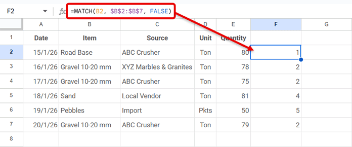
Google Sheets MATCH formula returning a self-match when the lookup value is part of the range

That’s not because another row matches—it’s because MATCH is matching the current row itself.

A Common but Flawed Workaround

A common idea is to split the range into two parts:

=MATCH(B2, B$1:B1, FALSE)

and

=MATCH(B2, B3:B, FALSE)

The first formula checks for a match above the current row, while the second checks below the current row. Together, they attempt to find the value anywhere in the column excluding the current row itself.

Using split-range MATCH formulas to avoid the current row in Google Sheets, showing unreliable results

While this can detect whether a match exists outside the current row, it has three serious drawbacks:

The relative position is no longer reliable
Combining both results into a single, meaningful position is messy
If the data starts from the first row (no header row), this approach breaks, because the “above row” range cannot be constructed safely.

Because of these limitations, the split-range approach is fragile and hard to maintain. While it may work for simple detection, it fails for position-based logic and breaks easily depending on how the data is structured—defeating the core purpose of using MATCH.

The Correct Way to Avoid Self-Matches in Google Sheets MATCH Formula

The proper solution is to remove the current row from the lookup range itself, then pass that adjusted range to MATCH.

Formula

=ARRAYFORMULA(
  MATCH(
    B2, 
    IF(ROW($B$2:$B)=ROW(),, $B$2:$B), 
    FALSE
  )
)

How It Works

In this array-based solution, the Google Sheets MATCH formula avoids self-matches by identifying the current row

ROW($B$2:$B)=ROW() identifies the current row
IF(...,,range) removes that value from the lookup array
MATCH searches the remaining values only
The returned position is correct and relative
ARRAYFORMULA is required because the IF(ROW()=ROW(),,range) expression generates an array, and MATCH needs that array to be explicitly materialized so it can evaluate all rows correctly.

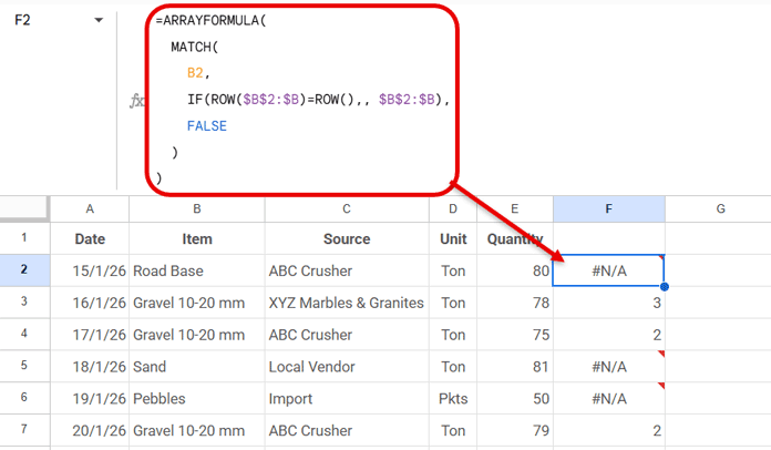
Google Sheets MATCH formula excluding the current row using ARRAYFORMULA to avoid self-matching

This works reliably in Google Sheets, including when copied down the column.

Using This Logic in Conditional Formatting

You can use the Google Sheets MATCH formula in conditional formatting to avoid self-matches, but only in specific cases.

If the search key exists in the lookup range and you want the relative position in a column, you can calculate it in a helper column using MATCH.
Then you can use that relative position in conditional formatting, for example:

=ISNUMBER(F2)

where F2 contains the relative position returned by MATCH.

However, if your goal is only to highlight duplicates, using MATCH is unnecessary. A simpler and faster approach is:

=COUNTIF($B$2:$B, B2) > 1

Use MATCH in conditional formatting only when you need the relative position; for simple duplicate highlighting, COUNTIF is sufficient.

Conclusion

We’ve seen how to avoid self-matches in the Google Sheets MATCH formula using an array-based approach.

COUNTIF → best for detecting duplicates
MATCH → best when you need relative position
Self-matches occur because the search key is part of the lookup array
The clean solution is to exclude the current row from the lookup array
Array-based exclusion is more reliable than split-range logic

If you understand why MATCH behaves this way, you’ll know when to use it—and when not to.