Average Array Formula Across Rows in Google Sheets

An average array formula across rows must return a row-wise average in Google Sheets. The AVERAGE function doesn’t expand its results—so how do we handle this?

We’ll use the BYROW function with a LAMBDA to return the average row by row. If you want to exclude zeros, simply replace AVERAGE with AVERAGEIF.

If you think BYROW is the only way to get a row-wise average in Google Sheets, think again — you can use DAVERAGE too. Although designed for structured databases, it can be adapted to unstructured ranges using helper functions and transposition.

This tutorial breaks it down into the simplest possible steps, so you can easily implement it in your Google Sheets.

Sample Data

Assume you have the following data in cells B1:E:

	Jan	Feb	Mar
Bed Frame	75	75	75
Bookshelf	0	96	90
Dining Table	45	55	65
Office Chair	0	10
Sofa Set		80	70

Let’s calculate the row-by-row average for each product. We’ll start with formulas where only the row end is open, i.e., future rows are included dynamically.

Average Array Formula Across Rows Including Zero

Method 1: BYROW with AVERAGE

Place the following formula in cell F2:

=BYROW(C2:E, LAMBDA(row, IFERROR(AVERAGE(row))))

This will return the average of each row, including zeros.

Row-wise average including zeros using an open-ended range

Formula Breakdown

BYROW(C2:E, ...): Applies the LAMBDA function row by row.
LAMBDA(row, ...): Treats each row independently.
AVERAGE(row): Computes the average of the current row.
IFERROR(...): Returns blank for empty rows.

Method 2: DAVERAGE

An alternative formula without using LAMBDA:

=ArrayFormula(IFERROR(
   DAVERAGE(
      VSTACK(SEQUENCE(1, ROWS(C2:C)), TRANSPOSE(C2:E)), 
      SEQUENCE(ROWS(C2:C)), 
      VSTACK(IF(,,), IF(,,))
   )
))

Formula Breakdown

DAVERAGE is designed to calculate the average of each column (i.e., vertically). It won’t work directly for row-by-row averages. To work around this, we transpose the data so rows become columns. Then DAVERAGE can handle the calculation as if it were working on columns.

TRANSPOSE(C2:E): Turns rows into columns.
VSTACK(SEQUENCE(...), ...): Adds dummy headers for DAVERAGE.
SEQUENCE(ROWS(C2:C)): Specifies the “fields” (original rows).
IFERROR(...): Suppresses errors.

Average Array Formula Across Rows Excluding Zero

Whether to include or exclude zeros depends on the context—include them if they represent valid values (like zero sales), and exclude them if they indicate missing or irrelevant data.

Method 1: BYROW with AVERAGEIF

=BYROW(C2:E, LAMBDA(row, IFERROR(AVERAGEIF(row, ">0", row))))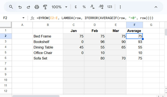

Row-wise average excluding zeros using an open-ended range

Formula Breakdown

AVERAGEIF(row, ">0", row): Ignores zeros in the average.
Remaining logic matches the BYROW + AVERAGE method.

Method 2: DAVERAGE with an IF Test

=ArrayFormula(IFERROR(
   DAVERAGE(
      VSTACK(SEQUENCE(1, ROWS(C2:C)), TRANSPOSE(IF(C2:E>0, C2:E, ))), 
      SEQUENCE(ROWS(C2:C)), 
      VSTACK(IF(,,), IF(,,))
   )
))

Formula Breakdown

IF(C2:E > 0, C2:E, ): Replaces zeros with blanks before transposing.
Remaining logic is the same as DAVERAGE including zero.

Average Each Row in a Fully Dynamic Range (Both Ends Open)

If your data grows horizontally and vertically, use a fully dynamic range.

You must:

Keep a blank column on the left (e.g., column A) so there’s room to insert the expanding average formula next to your dataset.
(Alternatively, you could enter the formula in a different sheet, but that’s usually less practical.)
Replace the fixed range (e.g., C2:E) with a dynamic one like:
INDIRECT("C2:"&ROWS(C2:C))
This ensures your formula adjusts automatically as new rows are added.

BYROW (Including 0)

=BYROW(INDIRECT("C2:"&ROWS(C2:C)), LAMBDA(row, IFERROR(AVERAGE(row))))

Dynamic row average including zeros (rows and columns open)

BYROW (Excluding 0)

=BYROW(INDIRECT("C2:"&ROWS(C2:C)), LAMBDA(row, IFERROR(AVERAGEIF(row, ">0", row))))

Dynamic row average excluding zeros (rows and columns open)

DAVERAGE (Including 0)

=ArrayFormula(IFERROR(
   DAVERAGE(
      VSTACK(SEQUENCE(1, ROWS(C2:C)), TRANSPOSE(INDIRECT("C2:"&ROWS(C2:C)))), 
      SEQUENCE(ROWS(C2:C)), 
      VSTACK(IF(,,), IF(,,))
   )
))

DAVERAGE (Excluding 0)

=ArrayFormula(IFERROR(
   DAVERAGE(
      VSTACK(SEQUENCE(1, ROWS(C2:C)), TRANSPOSE(IF(INDIRECT("C2:"&ROWS(C2:C))>0, INDIRECT("C2:"&ROWS(C2:C)), ))), 
      SEQUENCE(ROWS(C2:C)), 
      VSTACK(IF(,,), IF(,,))
   )
))

FAQs

Can I use AVERAGE without BYROW for arrays across rows?

No. AVERAGE returns a single value for the whole range. BYROW is needed to apply the function row-wise.

What if my data changes frequently?

Use dynamic ranges like INDIRECT("C2:"&ROWS(C2:C)) to automatically adapt.

What’s the difference between including and excluding 0s?

Include 0s when zeros are meaningful (e.g., “no sale”).
Exclude 0s when zeros indicate missing or non-relevant data.

Why does DAVERAGE require VSTACK and TRANSPOSE?

DAVERAGE is designed for columns. TRANSPOSE turns rows into columns. VSTACK adds a dummy header row needed for DAVERAGE to work.

What if I have a very large dataset?

If BYROW causes performance issues on large datasets, it’s best to avoid open-ended ranges. Instead, stick with static ranges like A1:E1000 to reduce overhead and improve performance.

Are there any other alternatives?

You can use MMULT or QUERY to average rows, but they are less flexible. QUERY can fail with blank cells, and MMULT works best with fixed-size ranges.

Resources

14 COMMENTS

Kevin October 27, 2022 At 2:48 pm

Hi Prashanth,

Thank you for the advice you provided in your article. I successfully used your formula (Including 0s).

What numbers do I need to change in this formula to calculate averages over more than three columns, let’s say five columns, for example?

Kind regards,
Kevin

- Prashanth October 28, 2022 At 11:22 am
  
  Hi, Kevin,
  
  I know you may have already tried replacing all B2:D with B2:F and B2:D2 with B2:F2 in the formula.
  
  But that’s not enough!
  
  You must also replace 3 in the Array_Constrain part of the formula with 5.
  
  Also, there is a much simpler solution now using BYROW with AVERAGE. I’ve updated the post!
  
DeLa June 22, 2022 At 3:57 am

Thanks for your response. After following your suggestion, I found that my issue was not with the range references (which translate fairly directly when moved); instead, it was a failure to expand the number of columns for ARRAY_CONSTRAIN to match my data set.
Many thanks for your wonderful and helpful content.

DeLa June 18, 2022 At 9:24 am

Greetings,

Many thanks for this helpful post.

If the data I want to evaluate starts in row 11 with column headers and row 12 with data, what adjustments do I need to make for the formula to work?

- Prashanth June 19, 2022 At 8:50 am
  
  Hi, DeLa,
  
  To get the formula for your data range, please do as follows.
  
  1. Create my sample sheet and apply the formula.
  2. Insert 10 rows at the top.
  3. Copy that formula to your data range.
  
Josh April 6, 2022 At 1:07 am

Personally, I think it’s much simpler to use this formula:

=ARRAYFORMULA((A:A+B:B+C:C+D:D)/4)

- Prashanth April 6, 2022 At 11:17 am
  
  Hi, Josh,
  
  The formula may break when you insert/delete columns.
  
Emily April 9, 2021 At 4:04 am

Thank you! Worked great.

Emily April 7, 2021 At 3:17 am

Hi Prashanth,

Thank you! That worked beautifully! Is there a way to keep the average to 2 decimal places?

Thanks again.

Emily

- Prashanth April 7, 2021 At 9:05 am
  
  Hi, Emily,
  
  Use ROUND() with the formula as below.
  
  =ArrayFormula({"LA: Listening & Speaking Average"; round(iferror(DAVERAGE(TRANSPOSE({sequence(rows(E2:E),1),E2:M}), sequence(rows(E2:E),1),{IF(,,);IF(,,)})),2)})
  
Emily April 2, 2021 At 10:12 pm

Hi Prashanth,

Thank you for the quick reply!

Here is a link to my spreadsheet: — link removed by admin —

Please feel free to edit as you wish. The form is not public nor live.

Thank you again for your help!

- Prashanth April 4, 2021 At 1:33 pm
  
  Hi, Emily,
  
  Thanks for sharing your sheet with Edit access.
  
  I’ve inserted the below DAVERAGE in cell AC1.
  
  ={"LA: Listening & Speaking Average";iferror(ArrayFormula( DAVERAGE(TRANSPOSE({sequence(rows(E2:E),1),E2:M}), sequence(rows(E2:E),1),{IF(,,);IF(,,)})))}
  
  I’ll write the tutorial soon and let you know by reply below.
  
  Another requirement is the IF logical test. I have converted the AD2:AD formula into an array formula. Please find that in cell AD1.
  
  I hope you can follow the formulas and replace other similar formulas.
  
Emily March 25, 2021 At 11:44 pm

Hi Prashanth,

Thank you for this article. I work with a K-6 school and I’ve created a form to serve as an assessment our teachers fill out for students. I would love some advice on calculating the average across rows as the form responses come in.

By no means am I a developer, so I get a bit lost in the complex formulas you use here. I attempted to tailor the formula to my spreadsheet but it didn’t work.

Any advice would be much appreciated! I can share my document if you’d like.

Thanks!

Emily

- Prashanth March 26, 2021 At 5:47 pm
  
  Hi, Emily,
  
  Feel free to share your sheet. Leave the link of your editable sheet (you can make a sample and share) via an answer to this thread.
  
  I won’t publish the link.
  
  In the sheet, explain what you want and also show me your hand entered (expected) result. I’ll try my best.