


")


")

")
")
 in Excel & Google Sheets")


You can avoid copy-pasting (or dragging) a formula down or across a sheet by using array formulas. An array formula sits in a single cell but automatically returns results across multiple rows or columns.
While this approach is powerful and convenient, it must be used carefully. Poorly designed array formulas can significantly slow down Google Sheets and make it feel unresponsive. In fact, many performance issues reported by users can be traced back to common ArrayFormula mistakes that slow down Google Sheets.
In this post, we’ll look at the most common array formula mistakes that cause performance problems and explain how to avoid them. The concepts discussed here apply not only to rows, but also to columns when array formulas are used horizontally.
TL;DR: Common ArrayFormula Mistakes and How to Fix Them
| Mistake | Why it Sinks Performance | The Better Way |
|---|---|---|
| Open Ranges (B2:B, C2:C, etc.) | Processes thousands of unnecessary empty rows, causing slow recalculations | Limit ranges (e.g., B2:B1000) or use IF short-circuits |
Using "" Instead of True Blanks | Forces Google Sheets to “fill” empty rows, adding unnecessary processing | Use IF(condition,,result) to return true blanks |
| Recalculating the Same Expression Multiple Times | Every repeated calculation inside ARRAYFORMULA multiplies workload, slowing the sheet | Use LET to store the result and reference it multiple times |
| Nested Volatile Functions (TODAY(), NOW(), RAND(), RANDBETWEEN()) | Every row becomes a volatile dependency, triggering massive recalculation chains | Put the volatile function in a helper cell and reference it inside the array formula |
| Using Heavy MMULT Formulas for Running Totals | Creates a large helper matrix, causing quadratic memory growth ($N^2$) | Use SUMIF, SCAN, or optimized linear formulas |
| Using Lambda-Based Functions Inefficiently (MAP, BYROW, BYCOL) | Rebuilding arrays for every row (FILTER inside LAMBDA) can scale poorly | Use vectorized functions like SUMIFS inside LAMBDA instead of FILTER |
| Using LAMBDA Functions When Not Needed | Adds unnecessary complexity without performance benefits | Use simple ARRAYFORMULA or native aggregation formulas |
Types of Array Formulas in Google Sheets (and Why Some Are Slower)
Broadly, array formulas fall into two categories:
1. Converting a regular formula into an array formula
This is done by using array references and either:
- Entering the formula as an array formula (Ctrl + Shift + Enter on Windows or Cmd + Shift + Enter on Mac), or
- Wrapping the formula with the ARRAYFORMULA function.
2. Using lambda-based functions
Functions like MAP, BYROW, or BYCOL apply the same logic to each row, column, or cell in an array.
Let’s start with the first type.
Converting a Regular Formula into an Array Formula
Placing the Formula in the Wrong Row (or Column)
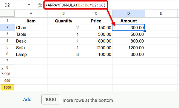
Assume you have quantities in column B and rates in column C, starting from row 2. In other words, the data range is B2:C6.
You can use the following formula in cell D2:
=ARRAYFORMULA(B2:B6*C2:C6)This multiplies quantities by their corresponding rates and does not cause any performance issues.
As your data grows, you may want the formula to automatically include new rows. To achieve this, many users switch to open-ended ranges:
=ARRAYFORMULA(B2:B*C2:C)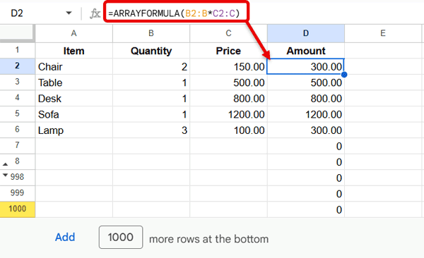
The Catch
When you use an open-ended array formula like this, you must place it in the starting row of the range (row 2).
If you accidentally place the formula in row 3 or below, Google Sheets tries to expand the result downward, inserts empty rows at the bottom of the sheet, and returns a #REF! error. You may then move the formula back to row 2 to fix the error—but the inserted empty rows remain.
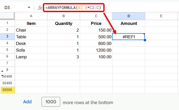
Those unused rows are still processed by Google Sheets. Over time, this becomes one of the classic ArrayFormula mistakes that slow down Google Sheets, as the sheet unnecessarily recalculates hundreds or even thousands of empty rows.
The same behavior applies when array formulas are used across columns with open-ended column ranges.
Using "" (Empty Text) Instead of True Blanks
Let’s consider the same array formula again.
You may notice that it returns trailing zeros due to empty rows. To remove them, you might be tempted to use a logical test like this:
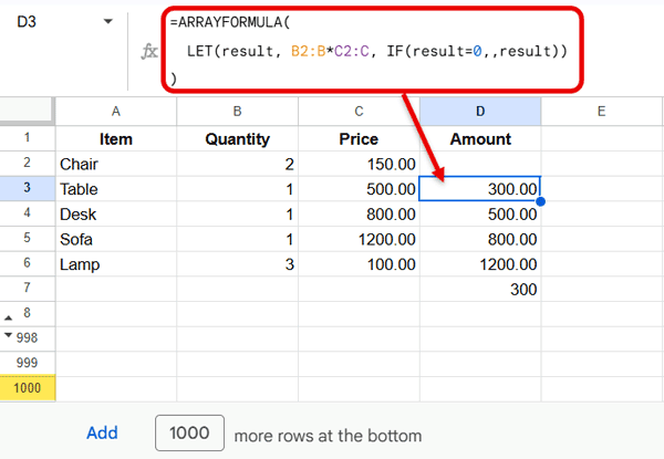
=ARRAYFORMULA(
  LET(result, B2:B*C2:C, IF(result=0,"",result))
)
Here, the LET function assigns the name result to the array calculation, and the IF function returns an empty string ("") when the result is zero.
Why This Is a Problem
- If the formula is entered in the starting row, it works fine.
- If it is entered lower down, it returns a
#REF!error and inserts empty rows at the bottom of the sheet.
Interestingly, if you replace the empty string with a true blank, the problem disappears:
=ARRAYFORMULA(
  LET(result, B2:B*C2:C, IF(result=0,,result))
)
or
=ARRAYFORMULA(
  LET(result, B2:B*C2:C, IF(result=0,IF(,,),result))
)
In these cases, Google Sheets does not insert empty rows at the bottom because the formula is not returning any value at all where the result is zero.
Key Takeaway
When using array formulas with open-ended ranges—either down rows or across columns—ensure the formula returns true blanks for empty cells.
Returning empty text ("") may look harmless, but it can cause Google Sheets to insert unnecessary rows or columns, leading to long-term performance issues.
This is a subtle but serious ArrayFormula mistake that slows down Google Sheets over time.
Using IF Short-Circuits to Skip Empty Rows
Another subtle way to improve performance when using open-ended ranges is to short-circuit calculations with IF. This prevents Google Sheets from calculating empty rows unnecessarily.
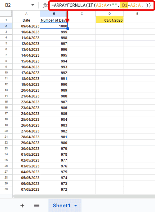
Example:
=ARRAYFORMULA(IF(B2:B<>"", B2:B*C2:C, ))Here, IF(B2:B<>"", …, ) checks if a cell in column B is not empty. Only non-empty rows are calculated, and empty rows are returned as true blanks. This reduces unnecessary processing and speeds up your sheet.
Tip: Combine this with placing your formula in the starting row and returning true blanks for the most efficient array formulas.
Recalculating the Same Expression Multiple Times Inside ARRAYFORMULA
Google Sheets has improved tremendously over the last few years, and one of the most important additions is the LET function.
LET allows you to assign a name to an expression and reuse it within the same formula. This helps in two ways:
- It makes formulas easier to read
- It prevents Google Sheets from recalculating the same expression multiple times
When this happens inside an ARRAYFORMULA, the performance impact becomes much more noticeable.
Using LET to Avoid Repeated Calculations
=ARRAYFORMULA(
  LET(result, B2:B*C2:C, IF(result=0,,result))
)
What happens here:
B2:B*C2:Cis calculated once- The result is stored in the variable
result - The
IFcondition referencesresult
This approach is efficient and scales well.
The Same Formula Without LET (Not Recommended)
=ARRAYFORMULA(
  IF(B2:B*C2:C=0,,B2:B*C2:C)
)
Internally, Google Sheets evaluates:
B2:B*C2:Cfor the logical testB2:B*C2:Cagain for the result
That means the same array calculation is performed twice for every row.
Why This Slows Down Google Sheets
ARRAYFORMULAalready expands calculations- Repeating expressions multiplies the workload
- As data grows, unnecessary recalculation becomes expensive
Even simple formulas can cause noticeable lag when repeated across large arrays.
Nesting Volatile Functions Inside ARRAYFORMULA
Another common ArrayFormula mistake that slows down Google Sheets is nesting volatile functions such as:
TODAY()NOW()RAND()RANDBETWEEN()
inside an ARRAYFORMULA.
On their own, these functions are usually harmless. The problem appears when they are evaluated once per row or column.
Example
=ARRAYFORMULA(IF(A2:A<>"", TODAY()-A2:A, ))Every time the sheet recalculates, TODAY() is applied to every row in the array. If the range spans hundreds or thousands of rows, this triggers a large recalculation chain and significantly slows down the sheet.
Better Approach
- Enter
=TODAY()in a helper cell - Reference that cell inside the array formula
This ensures the volatile function is evaluated only once and prevents the formula from being volatile across the array. When TODAY() is inside the array, Google Sheets treats every single row as a volatile dependency, increasing recalculation overhead.
Using the Wrong Formulas
Another major performance issue comes from using computational workarounds when simpler, optimized functions already exist.
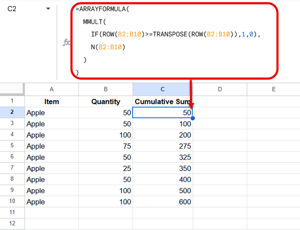
Example: Running Total Using Matrix Multiplication
=ARRAYFORMULA(
  MMULT(
    IF(ROW(B2:B10)>=TRANSPOSE(ROW(B2:B10)),1,0),
    N(B2:B10)
  )
)
This returns a running total—but it is extremely resource-intensive.
Why This Formula Is Inefficient
- Large helper matrix
1,000 rows create a 1,000 × 1,000 matrix (1 million cells). - Heavy MMULT calculations
Every row interacts with every other row, causing quadratic growth. ARRAYFORMULAmultiplies the recalculation cost
Any change forces the entire matrix to recalculate.
A Much Lighter Alternative
=ARRAYFORMULA(
  SUMIF(ROW(B2:B10), "<="&ROW(B2:B10), B2:B10)
)
This approach avoids matrices entirely and scales linearly.
Even Better with SCAN:
=SCAN(0, B2:B10, LAMBDA(acc, val, acc+val))Using Lambda-Based Functions
Note: If you’re not familiar with LAMBDA functions, you can still benefit from the earlier examples—this section is mainly for advanced users who want more flexible array calculations.
Lambda-based functions such as MAP, BYROW, and BYCOL are useful when regular array formulas cannot expand.
However, using inefficient logic inside an unnamed LAMBDA can hurt performance.
Example: Running Total by Category
=ARRAYFORMULA(
  MAP(
    B2:B,
    LAMBDA(area,
      SUMIFS(C2:C, B2:B, area, ROW(B2:B), "<="&ROW(area))
    )
  )
)
vs
=MAP(
  B2:B,
  C2:C,
  LAMBDA(area, amount,
    SUM(FILTER(C2:amount, B2:area=area))
  )
)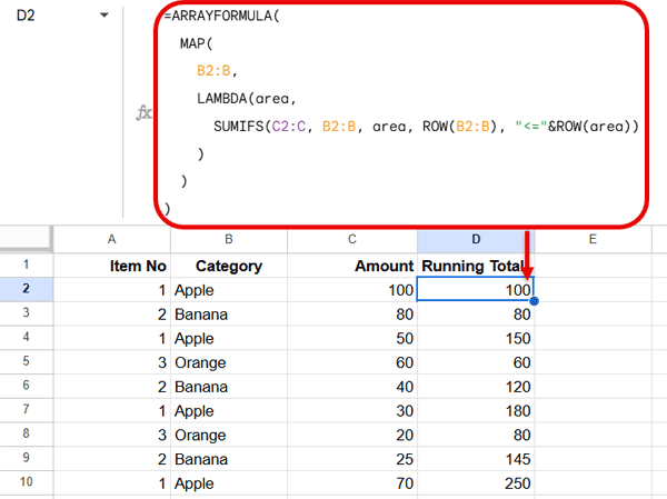
The first formula is more efficient because SUMIFS is a vectorized function in Google Sheets. It operates directly on entire ranges using the spreadsheet engine’s optimized aggregation logic.
The second formula rebuilds a filtered array inside an unnamed LAMBDA for every row. Each FILTER call creates a new intermediate array in memory, which scales poorly as the data grows.
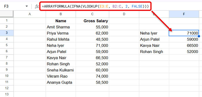
Using LAMBDA Functions When They’re Not Necessary
LAMBDA functions are powerful—but unnecessary use is another subtle ArrayFormula mistake that slows down Google Sheets.
=ARRAYFORMULA(IFNA(VLOOKUP(E3:E, B2:C, 2, FALSE)))is already sufficient.
Using:
=ARRAYFORMULA(
  BYROW(E3:E, LAMBDA(r, IFNA(VLOOKUP(r, B2:C, 2, FALSE))))
)
adds complexity without any performance benefit.
Final Thoughts
Array formulas amplify both good and bad design choices. Limiting ranges, avoiding unnecessary recalculation, choosing optimized functions, and understanding how Google Sheets processes arrays can make a huge difference.
By avoiding these ArrayFormula mistakes that slow down Google Sheets, you can build faster, cleaner, and more scalable spreadsheets—no matter how large your data grows.