Array Formula to Allocate Amounts into Monthly Columns in Google Sheets

When managing budgets, projects, or expenses in Google Sheets, you often need to allocate amounts into monthly columns to get a clear, month-by-month breakdown. Doing this manually for multiple rows and months can be time-consuming and error-prone. That’s where using an array formula to allocate amounts into monthly columns in Google Sheets comes in — it automates the process and scales effortlessly.

In this tutorial, we’ll explore two common methods to allocate amounts across monthly columns using array formulas:

Equal monthly allocation – The total amount is split evenly across all months in the date range.
Prorated allocation by days – The amount is split based on the actual number of days in each month between the start and end dates, giving a more precise allocation.

By the end, you’ll have working array formulas for both methods and know exactly when to use each for your needs.

Table of Contents

Preparing Your Data to Allocate Amounts into Monthly Columns in Google Sheets

Before you begin, decide whether you want equal monthly allocation or prorated allocation based on days. This decision changes one key column in your data setup.

For equal monthly allocation, your data should include:

Description
Start Date
End Date
Total Amount
Number of Months

For prorated allocation, the last column changes to:

Number of Days

In both cases, you’ll also have monthly columns — typically 12 columns from Jan to Dec — which will contain the allocated amounts.

Let’s start with the simpler option: equal monthly allocation.

Equal Allocation into Monthly Columns with Array Formula in Google Sheets

Here’s a sample dataset in A1:E5. Column E calculates the number of months:

=ArrayFormula(IFERROR(DATEDIF(EOMONTH(B2:B, -1)+1, EOMONTH(C2:C, -1)+1, "M") + 1))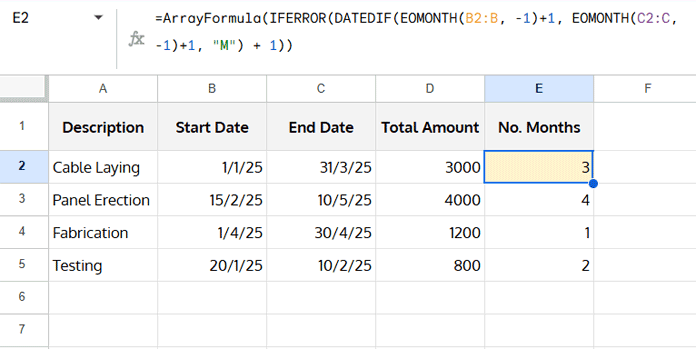

Sample dataset for allocating amounts into monthly columns in Google Sheets with Number of Months calculated

Note: This formula counts any month touched by the task as a whole month — even if it’s partial.

Setting Up Monthly Columns in Google Sheets

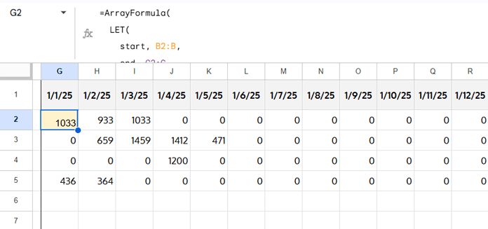
In G1:R1, enter month start dates from 1-Jan-2025 to 1-Dec-2025.

Array Formula for Equal Allocation into Monthly Columns

In G2, enter:

=ArrayFormula(
  LET(
    start, B2:B,
    end, C2:C,
    amt, D2:D,
    tm, E2:E,
    m, G1:R1,
    em, EOMONTH(m, 0),
    alm, (em >= EOMONTH(start, 0)) * (em <= EOMONTH(end, 0)),
    IFERROR(amt / tm * alm)
  )
)

Array formula for equal allocation into monthly columns in Google Sheets

Explanation:

start, end, amt, tm: Pulls start dates, end dates, amounts, and total months.
m: Month start dates from the header row.
em: End-of-month dates for each month column.
alm: A logical array that checks if each month (em) falls between the start and end months for each row. It returns 1 if true, 0 otherwise.
The final part amt / tm * alm divides the total amount by the number of months (tm) and multiplies it by the allocation mask (alm), effectively distributing the amount equally across the months involved.
IFERROR handles any possible errors gracefully.

This formula fills all monthly columns in one go.

Prorated Allocation into Monthly Columns by Days Using Array Formula in Google Sheets

For prorated allocation, instead of Number of Months, calculate Number of Days in column E:

=ArrayFormula(IF(B2:B, DATEDIF(B2:B, C2:C, "D") + 1,))

Sample dataset for prorated allocation by days with Number of Days calculated in Google Sheets

Array Formula for Prorated Allocation into Monthly Columns

In G2, enter:

=ArrayFormula(
  LET(
    start, B2:B,
    end, C2:C,
    amt, D2:D,
    td, E2:E,
    m, G1:R1,
    em, EOMONTH(m, 0),
    idStart, IF(em = EOMONTH(start, 0), start, EOMONTH(m, -1) + 1),
    idEnd, IF(em = EOMONTH(end, 0), end, em),
    ndays, idEnd - idStart + 1,
    alm, (em >= EOMONTH(start, 0)) * (em <= EOMONTH(end, 0)),
    IFERROR(ndays * alm * amt / td)
  )
)

Array formula for prorated allocation into monthly columns in Google Sheets

Explanation:

idStart – The actual start date for the current month:
idEnd – The actual end date for the current month:
- If the month contains the task’s end date, use that end date.
- Otherwise, use the last day of the month (em).
ndays – Number of days in the current month that the task spans.
alm – Allocation Month flag: 1 if the month falls between the start and end months, 0 otherwise.
ndays * alm * amt / td – Prorated allocation:
- Takes the days in this month (ndays),
- Multiplies by the allocation flag (alm),
- Scales by the daily rate (amt / td).
IFERROR(…) – Prevents errors for blank rows or months without allocation.

Equal vs. Prorated Allocation into Monthly Columns — Which Should You Use in Google Sheets?

Both Equal Allocation and Prorated Allocation have their place, depending on how you want to distribute your amounts across months. Here’s how to decide:

Scenario	Recommended Method	Why
Simple, uniform split across months (e.g., rent, subscription, retainer)	Equal Allocation	Easiest to set up, ensures each month in the range gets the same amount regardless of start/end days.
Partial months involved and accuracy matters (e.g., salaries, project billing, utilities)	Prorated Allocation	Calculates each month’s share based on the actual number of days covered, ensuring fairness in short or long months.
You don’t care about exact daily breakdown	Equal Allocation	Faster to compute and easier to read.
You need precise accounting for financial reporting	Prorated Allocation	Avoids over- or under-allocating amounts when periods start/end mid-month.

Tip:

If you start with Equal Allocation and later need more accuracy, you can easily switch to Prorated Allocation by just replacing the helper column formula and the allocation formula.
Keep in mind that prorated allocation involves more calculations, which can be slightly heavier for very large datasets.

Sample Sheet

Want to try it instantly? Here’s my sample sheet with formulas prefilled:

👉 Copy Sample Sheet