Array Formula to Allocate Amounts into Monthly Columns in Google Sheets

Published on

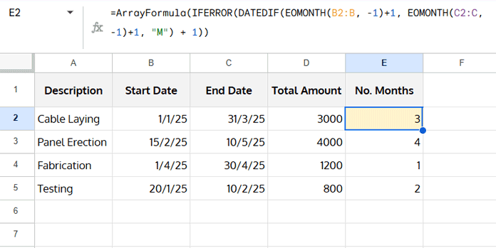
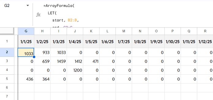
In Google Sheets, we can use an array formula to allocate amounts into monthly columns. It’s a tricky task!

I’m well familiar with Google Sheets. Writing an array formula for the monthly allocation of an amount is that much complicated?

Yes! It’s somewhat complicated. It seems simple. But it took me a couple of hours to solve the problem. There were a few hurdles in front of me that I eventually sorted out.

Let me explain the problem first. I have the following data.

Start Date: 15-Sep-2020 (in cell B4).

End Date: 15-Nov-2020 (in cell C4).

The amount to allocate is $500, which is in cell D4.

There are more rows with data. Let’s ignore that now. Based on the above data, I want to allocate the amount, i.e., $500, into the monthly columns September, October, and November.

Of course, I have an array formula to allocate the said amount into monthly columns in Google Sheets. But, for the time being, let’s forget about that for the sake of understanding the problem.

Monthly Allocation of Amounts (Understanding the Problem)

We can manually allocate the above amount into monthly columns as below in Google Sheets.

First, we must find the number of days between the start date and end date.

That’s quite easy. In cell F4, we can use the below formula to find the number of days between the start and end date.

=days(C4,B4)+1

Result: 62

Note: You can instead use the formula =datedif(B4,C4,"D")+1. Read more about these functions in my date function guide.

Then divide the amount to allocate with the above-returned number of days in cell F4 to get the per day amount.

=D4/F4

Result: 8.06

Here comes the complicated part. Based on the start and end date, we should allocate the amount as follows.

  • 16 days in September.
  • 31 days in October.
  • 15 days in November.

I mean, in September column 168.06, October column, 318.06, and in November column, 15*8.06.

That means the number of days might be different in the start month and end month. It may or may not be whole months. If you have more rows of data (see the below image), it’s going to be a headache.

How to solve this puzzle?

I have tried different combinations of formulas. After a few errors and trials, finally, I could successfully write an array formula to allocate amounts into monthly columns in Google Sheets.

Here is the output of my experiment (the values corresponding to the said example are in row # 4).

example to allocating amount into monthly columns

My array formula to allocate amounts into monthly columns is in cell H2. By residing in cell H2, this array formula returns the result in the range H2:M6!

In 5 steps, we can write an array formula to allocate the amount into monthly columns as above in Google Sheets.

Google Sheets Array Formula to Allocate Amounts into Monthly Columns

Sample Data and Basic Steps

For the sample data, please refer to the above image. The sample data is in columns B, C, D, and starting from row # 1.

Calculating Total Number of Days

In cell F2, insert the below formula to return the total number of days between the start date and end date.

=ArrayFormula(days(C2:C6,B2:B6)+1)

The result will be in F2:F6. So, before inserting the formula, you must ensure that F2:F6 is blank.

Preparing Month Wise Columns

We must use the end of the month dates to represent the months in the month column header row (H1:M1).

If it’s in text format, like “January, February…”, then we may want to use one more step to convert those values to the end of the month dates. So let’s use the end of the month dates to represent each month in the header row.

Further, I have chosen the months from August 2020 (31/08/2020) to January 2021 (31/01/2021). It is because my start dates and end dates in columns B and C are falling under that period.

But you can choose from January 2020 to December 2020 or as per your choice. My formula that allocates the amount into monthly columns is cross-year compatible. For the time being, you may please stick to the values provided in my sample data.

Let’s go to the first step to write the array formula to allocate amounts into monthly columns in Google Sheets.

Number of Days in First Row in Month Column (Step # 1)

It is the main step and the most complicated one.

All the other four steps are relatively simple. So I am breaking this step # 1 into a few sub-steps.

Sub-Step # 1

First, we will generate a row that replaces the H1:M1 dates as below. You will understand the purpose of this later.

If the month of H1:M1 = month of B2, year of H1:M1 = year of B2, and day of H1:M1 > day of B2, then replace that particular date in H1:M1 with the date in B2, else replace the dates in H1:M1 with eomonth($H$1:$M$1,-1)+1.

The EOMONTH formula here converts the end of the month dates in H1:M1 to starting dates in the corresponding months. I mean, 31/08/2020 will be converted to 01/08/2020.

=ArrayFormula(
     if(
        (month($H$1:$M$1)=month(B2))*
        (year($H$1:$M$1)=YEAR(B2))*
        (day($H$1:$M$1)>day(B2))=1,
        B2,
        eomonth($H$1:$M$1,-1)+1
     )
)
replacing month column date with matching start date

We want an array formula to allocate amounts into monthly columns in Google Sheets, but the above formula only covers the first row, right?

Don’t worry! We will later make it to cover all the rows.

Sub-Step # 2

It is the repetition of the above exercise.

Here there are two changes. Instead of B2 (start date), here we are going to use C2 (end-date).

Then instead of replacing the dates in H1:M1 with the end of the month dates, the formula is returning the dates in H1:M1 as it is.

That means;

If the month of H1:M1 = month of C2, year of H1:M1 = year of C2, and day of H1:M1 > day of C2, then replace that particular date in H1:M1 with the date in C2, else return the H1:M1 dates as it is.

For the time being I am inserting the sub-step # 2 formula in cell H8.

=ArrayFormula(
     if(
        (month($H$1:$M$1)=month(C2))*
        (year($H$1:$M$1)=YEAR(C2))*
        (day($H$1:$M$1)>day(C2))=1,
        C2,
        $H$1:$M$1
     )
)
replacing month column date with matching end date

Sub-Step # 3

To allocate amounts into monthly columns in Google Sheets, first, we must allocate the dates into monthly columns.

By deducting sub-step # 2 formula results with sub-step # 1 formula results, we can ‘partially’ achieve that.

To fully achieve this, we must convert the above formula to an array formula that covers start and end dates in multiple rows.

Generic Formula:

=ArrayFormula((sub_step_2 - sub_step_1)+1)

The +1 is to adjust the difference of 1 day, which happens when we deduct a future date from a past date.

Formula as per the Generic Formula:

=ArrayFormula(
   (
     if(
        (month($H$1:$M$1)=month(C2))*
        (year($H$1:$M$1)=YEAR(C2))*
        (day($H$1:$M$1)>day(C2))=1,
        C2,
        $H$1:$M$1
     )-
     if(
        (month($H$1:$M$1)=month(B2))*
        (year($H$1:$M$1)=YEAR(B2))*
        (day($H$1:$M$1)>day(B2))=1,
        B2,
        eomonth($H$1:$M$1,-1)+1
     )
   )+1
)

Replace cell H2 formula with the above one.

And also, remove the existing formula in cell H8 (because the above formula is the combination of both).

non-array formula to return month wise date allocated

Note:- If you see some other values in H2:M2 like dates or date values, format the range to number from the menu Format > Number > Number.

The formula above is the key to allocate the amount into monthly columns in Google Sheets.

Now to properly allocate the amounts month-wise, we can apply logical reasoning. Let’s go to that.

Number of Days Array Formula in Month Column (Step # 2)

First of all, let’s make the just above formula to cover the entire start and end dates. For that, replace B2 with B2:B6 and C2 with C2:C6.

Here, you may take utmost care. While replacing, don’t miss any references.

I am using the Find and Replace command to replace multiple references in formulas.

In Windows, use the shortcut key; Ctrl+H to open the “Find and replace” window and do as follows (see the below image).

replace multiple cell references in formula with find and replace

Similarly, replace C2 with C2:C6.

The H2 formula will now look like as below.

=ArrayFormula(
   (
     if(
        (month($H$1:$M$1)=month(C2:C6))*
        (year($H$1:$M$1)=YEAR(C2:C6))*
        (day($H$1:$M$1)>day(C2:C6))=1,
        C2:C6,
        $H$1:$M$1
     )-
     if(
        (month($H$1:$M$1)=month(B2:B6))*
        (year($H$1:$M$1)=YEAR(B2:B6))*
        (day($H$1:$M$1)>day(B2:B6))=1,
        B2:B6,
        eomonth($H$1:$M$1,-1)+1
     )
   )+1
)

Then highlight the range H2:M6 and format it to numbers (Format > Number > Number).

Note:- For the result, see the image below the next subtitle (range H2:M6).

Just select the total number of days by highlighting (selecting) F2:F6. On the footer near the Explore button, you can see the sum as 323.

Then highlight the distributed days in monthly columns in the range H2:M6. The sum would be 877!

Both the sum values should match, right?

It’s not matching because the above formula fills the number of days in all the monthly columns, which we don’t want.

To correctly allocate amounts into monthly columns, we want to remove the values in some columns based on start and end dates.

Finding the Proper Cells to Allocate the Amounts into Monthly Columns (Step # 3)

Using the following formula in cell H9, we can find the cells in which we want the number of days filled. That means identifying the cells to be filled with the allocation amount.

=ARRAYFORMULA(
     (H1:M1>=eomonth(B2:B6,0))*
     (H1:M1<=eomonth(C2:C6,0))
)

I guess this formula doesn’t need any explanation. See the image.

array formula to return month wise date to allocating amount

We should replace all the values 1 with the dates from the corresponding range in H2:M6 and 0s with blank.

It is the final hurdle we have to complete to allocate the amount into monthly columns in Google Sheets.

You can learn that in the next step. Actually, a simple step compared to step # 1 and step # 2 above.

Month Wise Distribution of Allocation Days (Step # 4)

To distribute the days month-wise in the correct columns and cells, follow the below generic formula.

=if(step_3_formula_result=1,step_2_formula,)

That means;

=ArrayFormula(if(H9:M13=1,H2:M6,))

Just replace cell ranges in the above formula with the corresponding formulas. Delete H2 and H9 formulas and insert the below-combined formula in cell H2. It’s as per the generic version above.

=ArrayFormula(
     if(
        (H1:M1>=eomonth(B2:B6,0))*
        (H1:M1<=eomonth(C2:C6,0))=1,
        (
           if(
              (month($H$1:$M$1)=month(C2:C6))*
              (year($H$1:$M$1)=YEAR(C2:C6))*
              (day($H$1:$M$1)>day(C2:C6))=1,
              C2:C6,
              $H$1:$M$1
           )-
           if(
              (month($H$1:$M$1)=month(B2:B6))*
              (year($H$1:$M$1)=YEAR(B2:B6))*
              (day($H$1:$M$1)>day(B2:B6))=1,
              B2:B6,
              eomonth($H$1:$M$1,-1)+1
           )
        )+1,
     )
)
example to allocating days into monthly columns

At this stage, anybody can easily allocate the amounts in D2:D6 to proper monthly columns in H2:M6.

Final Formula to Allocate Amounts into Monthly Columns in Google Sheets (Step # 5)

Here is my unique kind of formula that can allocate amounts into monthly columns in multiple rows by simply residing in cell H2.

I can make this step easier with one generic formula.

Generic Formula to Allocate Amount into Monthly Columns in Google Sheets:

=ArrayFormula(D2:D6/F2:F6*H2:M6)

or we can say;

=ArrayFormula(D2:D6/F2:F6*step_4_formula_result)

That means per day amount (amount divided by the total number of days) multiplied by month-wise distributed dates.

Let’s modify the H2 formula as above, and here is that final array formula to allocate the amount into monthly columns in Google Sheets.

=ArrayFormula(
     D2:D6/F2:F6*
     if(
        (H1:M1>=eomonth(B2:B6,0))*
        (H1:M1<=eomonth(C2:C6,0))=1,
        (
           if(
              (month($H$1:$M$1)=month(C2:C6))*
              (year($H$1:$M$1)=YEAR(C2:C6))*
              (day($H$1:$M$1)>day(C2:C6))=1,
              C2:C6,
              $H$1:$M$1
           )-
           if(
              (month($H$1:$M$1)=month(B2:B6))*
              (year($H$1:$M$1)=YEAR(B2:B6))*
              (day($H$1:$M$1)>day(B2:B6))=1,
              B2:B6,
              eomonth($H$1:$M$1,-1)+1
           )
        )+1,
     )
)

Conclusion

I have used closed ranges in the formula. I mean the formula is only for rows 2 to 6.

Can I make it for an open range so that the future start dates in columns B and C will be considered?

Yup! I can do that by changing B2:B6 with B2:B and C2:C6 with C2:C. That’s not enough! Use the following condition to avoid using blank rows at the end of the range.

if(len(D2:D),

Syntax:

=ArrayFormula(if(len(D2:D),step_5_formula,)

This formula you can find in my sample sheet shared below (tab name is ‘Copy of 5’).

array formula to allocate amount into monthly columns in Google Sheets

Further, In that sheet, I have modified H1:M1 to H1:S1 to cover the whole months in the year 2020.

So that you can use that sheet to allocate the amount into monthly columns in Google Sheets for a whole year. If you add more columns, change H1:S1 accordingly.

Finally, please note that the above formula won’t support excluding weekends in the monthly allocation.

That’s all. Enjoy!

Sample_Sheet_20820

Prashanth KV
Prashanth KV
Your Trusted Google Sheets and Excel Guide Prashanth KV brings a wealth of experience in Google Sheets and Excel, cultivated through years of work with multinational corporations in Mumbai and Dubai. As a recognized Google Product Expert in Docs Editors, Prashanth shares his expertise through insightful blogging since 2012. Explore his blog for practical tips and guidance on maximizing your spreadsheet skills.

Generate Unique Random Numbers in Excel with Dynamic Arrays

Unique random numbers refer to random numbers without duplicates. Generating such numbers is straightforward...

Lookup Previous Values Dynamically in Excel and Google Sheets

Sometimes, you may want to look up the previous values relative to the current...

Sort Data but Keep Blank Rows in Excel and Google Sheets

Using a dynamic array formula or the FILTER command, we can sort data and...

Lookup Values Under Categories in Excel and Google Sheets

We can use a combination of XLOOKUP and VLOOKUP in both Excel and Google...

More like this

XMATCH Row by Row: Finding Values Across a Range in Google Sheets

Using the BYROW function with XMATCH in Google Sheets allows us to match values...

Limit Formula Expansion to a Specific Row in Google Sheets

In this tutorial, I’ll explain how to limit the expansion of an array formula...

3-D Referencing Structured Data Tables in Google Sheets

When you have several tables within a single sheet—not across multiple sheets in a...

LEAVE A REPLY

Please enter your comment!
Please enter your name here

This site uses Akismet to reduce spam. Learn how your comment data is processed.