If you work with structured data in Google Sheets, you may want to display it in a hierarchical table instead of keeping everything in a flat list. For example, you might have three columns for Region, Country, and City and want them arranged in a clear three-column tree view in Google Sheets.

In this guide, we’ll build a Google Sheets hierarchical table using a single formula — no scripts required.

Step 1: Prepare Your Data

Start with a simple dataset containing three columns, such as Continent, Country, and Major Cities.

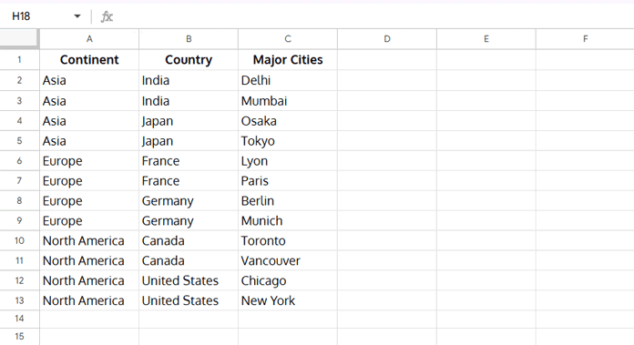
👉 Avoid leaving empty rows between records. If the top-level category is blank, the formula will skip its sub-categories and lowest-level values in the tree view.

So, in a 3-column hierarchical table, your three levels are:

1. Continent – top-level category
2. Country – sub-category under each continent
3. Major Cities – lowest level

Step 2: Understand the Hierarchy

The goal is to display your data like this:

This is a three-column tree view in Google Sheets. If you only provide two columns of data (for example, Continent and Country), the same formula will still work and return a 2-column hierarchical table.

Step 3: Use the Formula

In Google Sheets, you can generate a hierarchical table with a single formula by combining functions such as ARRAYFORMULA, FILTER, UNIQUE, VSTACK, HSTACK, SEQUENCE, and REDUCE.

Here’s the formula for creating a 3-column hierarchical table in Google Sheets:

=ArrayFormula( 
  LET( 
    topL, A2:A, 
    subCat, B2:B, 
    lowestL, C2:C, 
    stg_1, REDUCE(TOCOL(,1), TOCOL(UNIQUE(subCat), 1), 
              LAMBDA(a, v, VSTACK(a, HSTACK(v, VSTACK(, UNIQUE(FILTER(lowestL, subCat=v))))))), 
    stg_id, CHOOSECOLS(stg_1, 1), 
    stg_2, LOOKUP(SEQUENCE(ROWS(stg_id)), SEQUENCE(ROWS(stg_id))/(stg_id<>""), stg_id), 
    stg_3, XLOOKUP(stg_2, subCat, topL), 
    fnl, REDUCE(TOCOL(,1), TOCOL(UNIQUE(topL), 1), 
              LAMBDA(a, v, VSTACK(a, HSTACK(v, VSTACK(, FILTER(stg_1, stg_3=v)))))), 
    IFNA(fnl) 
  ) 
)

Step 4: Customize the Formula

When you use this formula for a three-column tree view, update the column ranges if your data is not in A2:C.

Replace:

• A2:A with the top-level category range
• B2:B with the sub-category range
• C2:C with the lowest-level range

👉 If your data is in a different sheet, include the sheet name. For example:
'Sheet1'!A2:A, 'Sheet1'!B2:B, and 'Sheet1'!C2:C.

Formula Explanation

The formula we used looks complex, but it’s easier to follow if we break it into stages. Each stage transforms the data step by step until we get a full Google Sheets hierarchical table in a clean three-column tree view.

Stage 1: Create the Sub-Category + Lowest Level Pair

stg_1, REDUCE(TOCOL(,1), TOCOL(UNIQUE(subCat), 1), 
              LAMBDA(a, v, VSTACK(a, HSTACK(v, VSTACK(, UNIQUE(FILTER(lowestL, subCat=v)))))))

This step produces a two-column hierarchy:

• Column 1 → each unique sub-category (Country in our example)
• Column 2 → the corresponding unique lowest-level values (Cities)

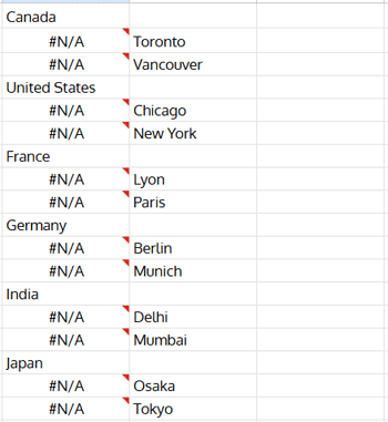
The trick here:

• FILTER pulls all cities for a country
• UNIQUE removes duplicates
• HSTACK joins the country with its cities
• VSTACK stacks everything neatly under each other

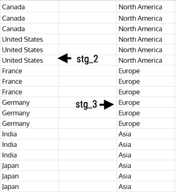
Stage 2: Fill Down the First Column

stg_id, CHOOSECOLS(stg_1, 1), 
stg_2, LOOKUP(SEQUENCE(ROWS(stg_id)), SEQUENCE(ROWS(stg_id))/(stg_id<>""), stg_id)

The first column in stg_1 includes #N/A padding introduced by the seeding/stacking step (it’s not just blank cells). This stage uses the classic LOOKUP fill down pattern to carry forward the last non-empty value, effectively ignoring the #N/A padding so every city row displays its country. This ensures every City is properly paired with its Country before we map back to Continents. (You’ll see the filled result in the Stage 3 screenshot.)

Stage 3: Map Countries Back to Continents

stg_3, XLOOKUP(stg_2, subCat, topL)

This step maps each filled-down sub-category in stg_2 to its corresponding top-level value (Continent). The result is a top-level column the same length as stg_2, which we’ll use to filter and group everything correctly in the final hierarchy.

Stage 4: Build the Final Hierarchy

fnl, REDUCE(TOCOL(,1), TOCOL(UNIQUE(topL), 1), 
              LAMBDA(a, v, VSTACK(a, HSTACK(v, VSTACK(, FILTER(stg_1, stg_3=v))))))

Here’s where everything comes together:

• Each unique Continent is taken
• Under it, all related Countries and Cities are stacked
• VSTACK ensures indentation-style spacing
• Finally, IFNA(fnl) removes padding errors (#N/A)

End result → a fully dynamic three-column tree view in Google Sheets. Anytime you add or remove data, the hierarchy updates automatically.

Additional Tip: Pivot Table–Like Layout

By default, the formula creates a tree view with indentation — each level is slightly offset so you can see the hierarchy more clearly.

If you prefer a pivot table–style layout, where all three levels (Continent → Country → City) align neatly in columns, you can tweak the formula a bit. The main change is removing the extra VSTACKs that insert blank rows for indentation. This way, the output looks more like a traditional pivot table.

Here’s the adjusted formula for that layout:

=ArrayFormula( 
  LET( 
    topL, A2:A, 
    subCat, B2:B, 
    lowestL, C2:C, 
    stg_1, REDUCE(TOCOL(,1), TOCOL(UNIQUE(subCat), 1), 
              LAMBDA(a, v, VSTACK(a, HSTACK(v, UNIQUE(FILTER(lowestL, subCat=v)))))), 
    stg_id, CHOOSECOLS(stg_1, 1), 
    stg_2, LOOKUP(SEQUENCE(ROWS(stg_id)), SEQUENCE(ROWS(stg_id))/(stg_id<>""), stg_id), 
    stg_3, XLOOKUP(stg_2, subCat, topL), 
    fnl, REDUCE(TOCOL(,1), TOCOL(UNIQUE(topL), 1), 
              LAMBDA(a, v, VSTACK(a, HSTACK(v, FILTER(stg_1, stg_3=v))))), 
    IFNA(fnl) 
  ) 
)

3-Column to 2-Column Hierarchical Table

If you only need two levels (e.g., Continent → Country), you can simplify the formula. Just provide data in two columns:

=ArrayFormula( 
  LET( 
    topL, A2:A, 
    subCat, B2:B, 
    stg_1, REDUCE(TOCOL(,1), TOCOL(UNIQUE(topL), 1), 
              LAMBDA(a, v, VSTACK(a, HSTACK(v, VSTACK(, UNIQUE(FILTER(subCat, topL=v))))))), 
    IFNA(stg_1) 
  ) 
)

This creates a 2-column hierarchical table without referencing an empty third column.

Resources

👉 Sample Google Sheet (3 tabs: Sample Data, Hierarchy, Pivot Style Hierarchy)

Related tutorials:

• How to Create a Tree Map Chart in Google Sheets
• How to Number Rows as 1, 1.1, 1.2, 1.3 in Google Sheets
• Hierarchical Numbering Sequences in Excel
• Hierarchical Number Sorting in Excel with Modern Functions