Excel offers multiple ways to accomplish tasks, and the simplicity of each approach depends on your familiarity with the application. Repeating a sequence of numbers in Excel is one such task, and it can be done with or without complex functions like LAMBDA. This tutorial introduces one of the easiest and most flexible ways to repeat a sequence of numbers in Excel.
You can repeat sequences of either integers or decimal values. For instance, you can create a sequence from 1 to n with a step of 1, or repeat a sequence from 0.25 to n with a step of 0.25. The starting value can be either a decimal or an integer, and you can control how many times each number in the sequence is repeated.

In this guide, we’ll use the Excel functions SEQUENCE, HSTACK, VLOOKUP, and TOCOL to create a flexible formula that repeats a sequence based on specified parameters. We’ll also set up our inputs so you can easily control the sequence length, repetition count, starting value, and increment value.
Step 1: Setting Up the Input Parameters
In cells A1:B4, set up your parameters as shown below:
| Parameter | Value |
| Unique sequence | 10 |
| Starting at | 1 |
| Increment by | 1 |
| Numbers up to | 3 |
Explanation of Parameters:
- Unique sequence: The total number of unique values in the sequence. For example, if this value is 10, the sequence will have 10 unique numbers.
- Starting at: The starting point of the sequence. This can be a decimal or integer (e.g., starting at 1).
- Increment by: The step value between numbers in the sequence. A step of 1 means each subsequent number is increased by 1.
- Numbers up to: The number of times each value in the sequence should be repeated. If this is set to 3, each number in the sequence will appear thrice.
Step 2: Formula to Repeat Sequence of Numbers in Excel
In cell D1, enter the following formula to repeat the sequence according to the parameters specified in column B:
=TOCOL(
   VLOOKUP(
      SEQUENCE(B1),
      HSTACK(SEQUENCE(B1), SEQUENCE(B1, 1, B2, B3)),
      2,
      SEQUENCE(1, B4, 0, 0)
   ),,FALSE
)
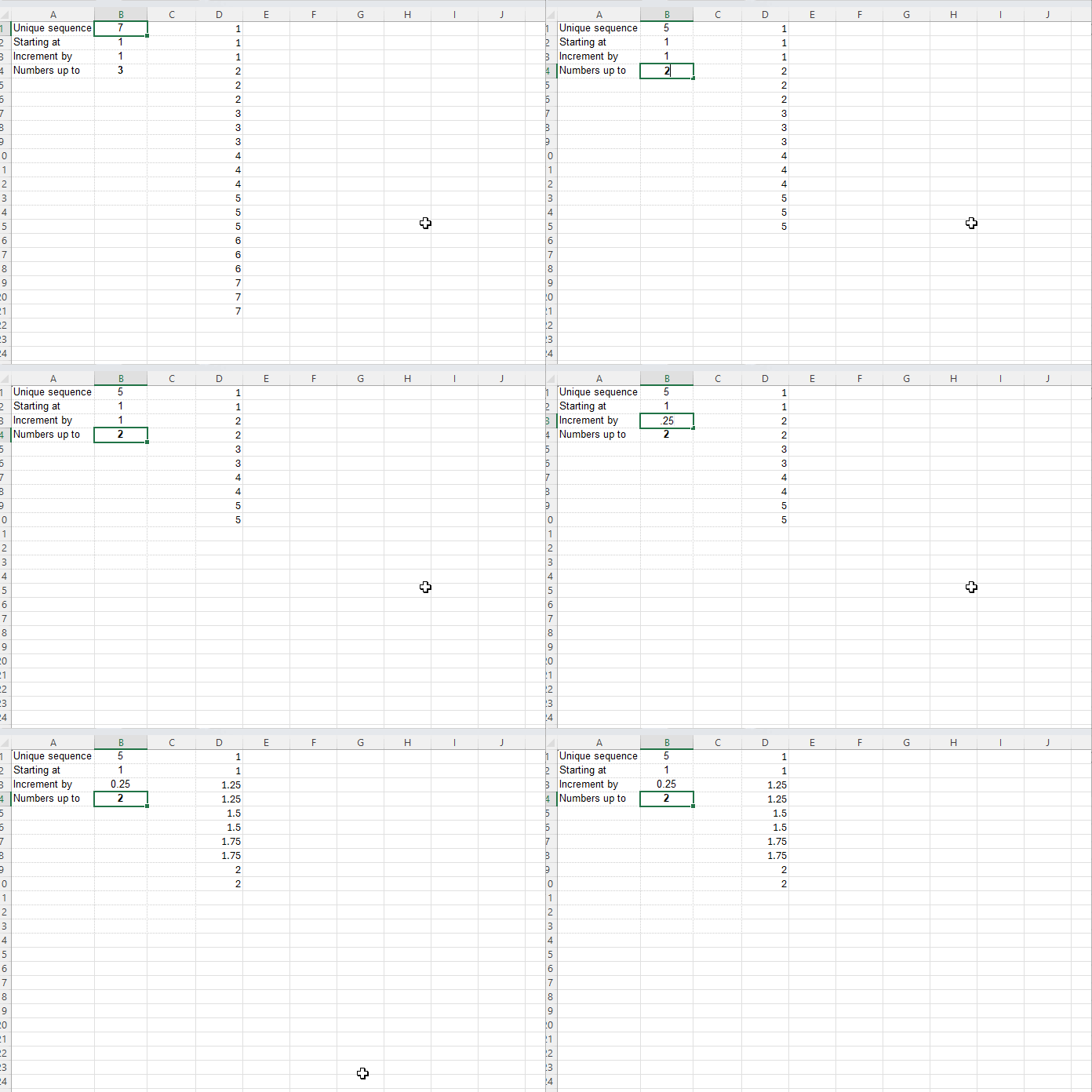
This formula will return a sequence like the following:
1
1
1
2
2
2
3
3
3
...
If you change the value in Numbers up to (cell B4) to 2, the output will change to:
1
1
2
2
3
3
...
If you set Starting at and Increment by to 0.25, the output will look like:
0.25
0.25
0.50
0.50
0.75
0.75
1.00
1.00
...
Note: If the results appear as integers, select the result range, go to the Home tab, and click Increase Decimal in the Number group to display the desired decimal places.
This formula is one of the best dynamic array solutions for repeating a sequence of numbers in Excel. It supports decimal, negative, and integer values without using LAMBDA, making it efficient and versatile.
Formula Breakdown
Let’s look at the key components of this formula:
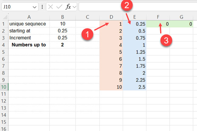
=SEQUENCE(B1)
This returns a sequence from 1 up to the number specified in cell B1 (the total unique sequence count).=SEQUENCE(B1, 1, B2, B3)
This generates a sequence starting at the value in Starting at (B2) and incrementing by the value in Increment by (B3), without repetitions.=SEQUENCE(1, B4, 0, 0)
This creates a sequence of zeros that repeats the values according to Numbers up to (B4).

How These Components Work Together
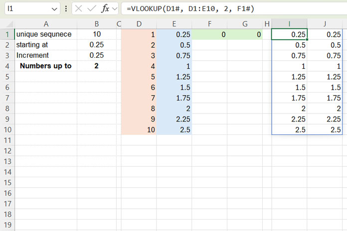
We use VLOOKUP to combine these components and create the repeated sequence. The syntax is:
VLOOKUP (lookup_value, table_array, col_index_num, [range_lookup])Where:
- lookup_value:
SEQUENCE(B1)– Component 1. - table_array:
HSTACK(SEQUENCE(B1), SEQUENCE(B1, 1, B2, B3))– combining Component 1 and Component 2. - col_index_num: 2 – instructs
VLOOKUPto return values from the second column in thetable_array. - range_lookup:
SEQUENCE(1, B4, 0, 0)– Component 3.
The VLOOKUP function searches down the lookup_value in the first column of the table_array and returns the corresponding value from the second column, as specified by col_index_num = 2.
This effectively returns Component 2 values as they are.
However, because range_lookup is defined by Component 3 (a sequence of zeros), it repeats each result the specified number of times. This is a clever VLOOKUP hack that many people aren’t aware of.

Finally, we use TOCOL to convert the 2D array output into a 1D array, creating the desired repeated sequence.
Why This Formula Works Well for Repeating a Sequence of Numbers
This formula provides an efficient and flexible way to repeat a sequence of numbers in Excel. It supports both decimal and integer values, avoids complex LAMBDA functions, and is optimized for performance.
If you want to create a repeating sequence of negative numbers, that’s also possible. For example, specifying Starting at -1 in cell B2 and incrementing by -1 in cell B3 will generate a negative sequence. The numbers will repeat according to the value specified in cell B4, and the number of unique sequences will follow the value in cell B1.
This approach is highly flexible and straightforward, not involving LAMBDA functions. Try it out yourself, and feel free to leave your valuable feedback!


