")
")


")


")

")
")
 in Excel & Google Sheets")


To remove the first two characters (whether they are letters or digits) from a cell in Excel, you can use the MID+LEN, LEFT+LEN, or REPLACE function. I prefer the REPLACE function.
If the cell content is a number, you might also use the VALUE function to ensure the result remains in a numeric format.
Removing the First Two Letters
The following formulas will remove the first two characters (letters) from the text in cell A2:
=IFERROR(RIGHT(A2, LEN(A2)-2), "")
TheLEN(A2)-2part calculates the total number of characters in cell A2 and subtracts 2. The RIGHT function then extracts the remaining characters from the right, effectively removing the first two characters.
This formula may return a#VALUE!error if the length of the string is less than 2. The IFERROR function handles this error by returning an empty string.=MID(A2, 3, LEN(A2))
The MID function extracts the characters starting from the third character (position 3) to the end of the string, as determined by the LEN function.=REPLACE(A2, 1, 2, "")
The REPLACE function removes 2 characters starting from the first character by replacing them with an empty string ("").
If the value in cell A2 is “NO145AZ1”, all of these formulas will return “145AZ1”.
Example
In the following examples, item codes are listed in the range A2:A10. Enter one of the formulas, preferably the REPLACE function, in cell C2 and drag it down to C10.
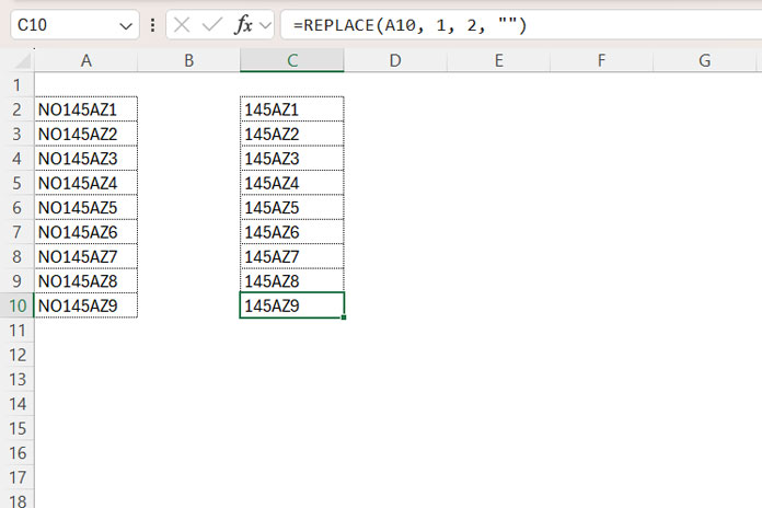
If your version of Excel supports dynamic arrays, you can simply enter the following formula in cell C2:
=REPLACE(A2:A10, 1, 2, "")The results will automatically spill down the column.
Now let’s see what changes we need to make to the formulas when you want to remove the first two digits.
Removing the First Two Digits
The formulas above remove the first two characters (letters or numbers). However, when the values are numbers, the output will be in text format.
To retain the numeric format, you should either multiply the result by 1 or use the VALUE function.
Assume cell A2 contains the number 123456. The output of the following formulas will be 3456 in number format.
=IFERROR(VALUE(RIGHT(A2,LEN(A2)-2)), 0)
=IFERROR(VALUE(MID(A2, 3, LEN(A2))), 0)
=IFERROR(VALUE(REPLACE(A2, 1, 2, "")), 0)
If the value is 5000, the result will be 0.
If cell A2 contains a number with fewer than 3 digits, the output will typically be an error. The IFERROR function replaces that error with 0.
Here is the recommended array formula to remove the first two digits for those using the latest versions of Excel with dynamic array support:
=IFERROR(VALUE(REPLACE(A2:A10, 1, 2, "")), 0)