")
")


")


")

")
")
 in Excel & Google Sheets")


We often use the OFFSET and XMATCH functions together to match a value in one column and return a corresponding value from another column in Excel. Additionally, we can use XMATCH to match multiple values and extract the intermediate values from another column.
When dealing with values between two points, the values to match may either both be distinct, or one value may be distinct while the other is repeated. Let’s explore these scenarios with examples of using OFFSET and XMATCH in Excel.
Example 1: OFFSET and XMATCH Basic Use in Excel
Imagine you have student names in column A and their total marks in column B. The range is A2:B4:
The following formula will return the marks of “Mike”:
=OFFSET(B2, XMATCH("Mike", A2:A4)-1, 0, 1, 1)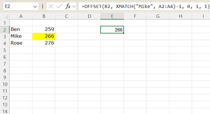
In this formula, OFFSET is used to return the value from a specified number of rows and columns away from a starting cell.
Syntax: OFFSET(reference, rows, cols, [height], [width])
The function XMATCH("Mike", A2:A4) finds the relative position of “Mike” in the range A2:A4, which is 2. Since Excel’s OFFSET uses zero-based indexing, we subtract 1 to get the correct row offset (rows).
The starting cell reference B2 (reference) is where the offset begins. If you change the reference to A2, the formula will return a value from column A instead.
This demonstrates the basic use of the OFFSET and XMATCH combination in Excel.
Example 2: OFFSET and XMATCH to Extract Values Between Two Distinct Values
In this example, the data includes student names as headers in column A, with their subject-wise marks listed below. Column B contains the corresponding marks. The range is A1:B13:
To extract all marks for “Mike” based on the names “Mike” and “Rose” as boundaries, use the following formula:
=OFFSET(B2, XMATCH("Mike", A2:A13), 0, XMATCH("Rose", A2:A13) - XMATCH("Mike", A2:A13) - 1, 1)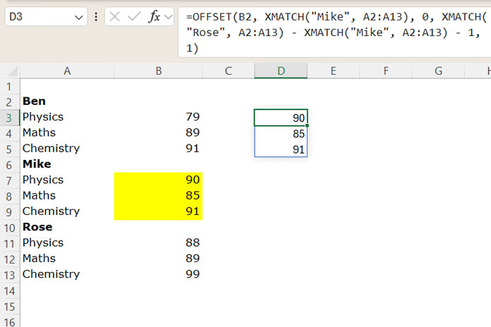
Here, XMATCH("Mike", A2:A13) locates the starting position of “Mike” (rows) in column A. Similarly, XMATCH("Rose", A2:A13) locates the starting position of “Rose”. The difference between these positions, minus 1, determines the height (number of rows) of the range to extract.
OFFSET starts at B2 (reference), moves down by the rows returned by XMATCH("Mike", A2:A13), and retrieves values from column B corresponding to the range between “Mike” and “Rose”.
This formula is useful for extracting intermediate values based on two distinct boundaries.
Example 3: OFFSET and XMATCH to Extract Values Between One Distinct Value and Another Duplicate Value
Sometimes, you may need to retrieve all marks for a student without specifying the name of the next student. For example, if you want all marks for “Rose” until the last subject “Chemistry,” use this formula:
=LET(
   xm_, XMATCH("Rose", A2:A13),
   xmo_1, OFFSET(A2, xm_, 0, 10),
   xm__, XMATCH("Chemistry", xmo_1),
   OFFSET(B2, xm_, 0, xm__, 1)
)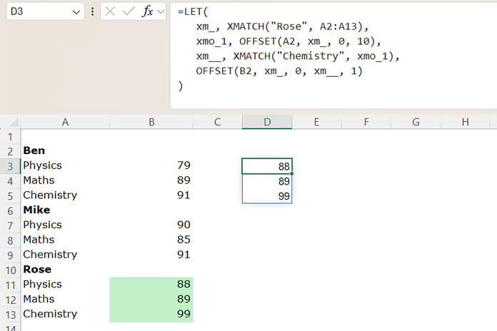
This formula uses LET to define intermediate variables and simplify the calculation.
The variable xm_ stores the position of “Rose” in column A, while xmo_1 offsets from A2 by this position and retrieves 10 rows (an arbitrary number larger than the expected rows). Then, xm__ calculates the position of “Chemistry” within this range.
Finally, OFFSET(B2, xm_, 0, xm__, 1) retrieves the marks for “Rose” up to “Chemistry.”
This approach is particularly useful when the second boundary value appears multiple times in the data.