There is no dedicated function in Excel to directly find the mode of comma-separated numbers stored as text within a single cell. However, in real-world scenarios—like survey data or grouped responses—you might need to extract the most frequently occurring number (mode) from such text-based lists.
So how can you calculate the mode of comma-separated numbers in Excel when the numbers are in a single text string?
We’ll use a formula-based approach combining TEXTSPLIT, VALUE, and the MODE.MULT or MODE.SNGL functions. Since functions like MODE.MULT expect numeric arrays and not text, we first need to split and convert the values.
In this tutorial, I’ll show you two methods:
- A drag-down formula to find the mode for each row individually.
- An array formula to return the modes for an entire column at once.
Note: These methods require Excel 365 or Excel 2021 with support for dynamic arrays.
Sample Data for Mode Calculation in Excel
Assume you conducted a product survey across different regions. Each response is recorded as a comma-separated list of numeric codes representing specific reasons:
| Code | Meaning |
| 1 | Too Expensive |
| 2 | Lack of Features |
| 3 | Slow Service |
| 4 | Poor Support |
| 5 | Technical Issues |
You’ve stored the responses region-wise as follows:
| Region | Response Codes |
| North | 1,2,1,1,1 |
| South | 3,3,1,3,4 |
| East | 1,1,5,4,4 |
| West | 3,3,4,4,1 |
Your goal is to find the most common response code (mode) in each row, i.e., the mode of comma-separated numbers in Excel.
Drag-Down Formula to Find the Mode of Comma-Separated Numbers in Excel
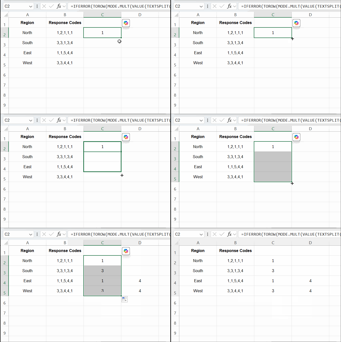
To calculate the mode for each cell individually, enter the following formula in cell C2 and drag down:
=IFERROR(TOROW(MODE.MULT(VALUE(TEXTSPLIT(B2,",")))),"")
Formula Explanation
TEXTSPLIT(B2, ","): Splits the comma-separated string into an array of text values.VALUE(...): Converts the text values to numbers.MODE.MULT(...): Returns the mode(s) from the numeric array (multiple modes if they exist).TOROW(...): Ensures the result appears as a single row, even if multiple modes are returned.IFERROR(..., ""): Prevents errors if there’s no mode (e.g., all values are unique).
Note: If you only need a single result, replace MODE.MULT with MODE.SNGL.
Dynamic Array Formula to Find the Mode of Comma-Separated Numbers in Excel
To calculate the mode from each cell in the range B2:B5 at once, use this dynamic array formula:
=DROP(
   IFNA(
      REDUCE(
         0, B2:B5,
         LAMBDA(acc, val,
            VSTACK(acc, IFERROR(TOROW(MODE.MULT(VALUE(TEXTSPLIT(val, ",")))), ""))
         )
      ), ""
   ), 1
)
How the Array Formula Works
REDUCE: Loops through the rangeB2:B5and builds the result row by row.TEXTSPLIT+VALUE: Splits and converts each string into a numeric array.MODE.MULT: Computes the mode(s) for each array.TOROW: Ensures the output remains in a single row per item.IFERROR(..., ""): Catches and suppresses any errors (such as no mode).VSTACK: Stacks each row result vertically.DROP(..., 1): Removes the initial zero used as the seed value inREDUCE.IFNA(..., ""): Handles any empty or error outputs.
Can You Use the Same Formula in Google Sheets?
No. While the logic is similar, the formulas are not interchangeable due to key differences:
| Excel | Google Sheets |
Uses TEXTSPLIT and VALUE | Uses SPLIT (automatically converts to numbers) |
IFERROR/IFNA require second argument | Second argument is optional |
Uses REDUCE for row-wise computation | Uses MAP instead |
In Excel, especially when using MODE.MULT with dynamic arrays, we need REDUCE and VSTACK to return per-row results.
Real-Life Use Case: Survey Response Analysis
Let’s say you’re analyzing survey responses collected from different regions. Each region’s data represents responses from multiple individuals, with each respondent selecting one reason for dissatisfaction. The responses were then compiled into a single cell per region as comma-separated numeric codes. To summarize the feedback, you want to identify the most frequently selected reason in each region.
Finding the mode of comma-separated numbers in Excel is ideal for such cases where grouped numeric responses—each representing a single response from multiple individuals—are stored as text in one cell.


