 in Google Sheets")

")

")


")


")


Adding a blank row after each category change in Excel is quite simple. You just need to follow three easy steps. This applies to physical data. If you want to achieve the same with the output of a dynamic array formula such as FILTER, a different approach is required. We will explore both options in this Excel tutorial.
To start with, we’ll consider the physical data. For example, let’s use the following sample data in the range B1:D11:
| A | B | C | D |
| Item | Grade | Qty | |
| Apple | I | 5 | |
| Apple | I | 5 | |
| Apple | II | 4 | |
| Apple | II | 5 | |
| Banana | I | 5 | |
| Banana | I | 5 | |
| Lettuce | III | 6 | |
| Mango | I | 5 | |
| Orange | I | 10 | |
| Orange | I | 10 |
Please note: To insert a blank row below each group, we need a blank column in front of the source data. Here, Column A serves that purpose.
Step 1: Numbering Groups with Identical Values
In column B, there are four categories: Apple, Banana, Lettuce, and Orange.
To number them sequentially—assigning 1 to Apple, 2 to Banana, 3 to Lettuce, and 4 to Orange—follow these steps:
In cell A2, enter the following formula and drag it down to A11:
=IF(B2<>B1, MAX(A$1:A1)+1, MAX(A$1:A1))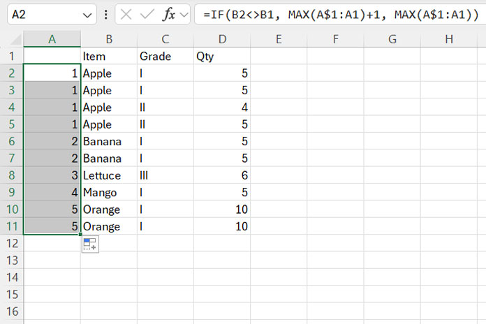
Explanation of the Formula:
The formula checks if the value in B2 is different from B1. If this condition is true (i.e., there’s a change in the category), it returns MAX(A$1:A1)+1, which increments the number for the new category.
For the first occurrence of each category, the formula will evaluate TRUE and assign a new number. For subsequent rows within the same category, the formula evaluates to FALSE, so it keeps the same number.
Still unclear? For instance, if B2 is different from B1, the formula returns MAX(A$1:A1)+1. Initially, A1 is empty, so it will be 0+1=1.
In the next row, if B3 is the same as B2, the formula returns the maximum value from the previous rows, which is 1.
When a category changes (for example, in row 5 where B6 is different from B5), the formula again evaluates to TRUE and returns MAX(A$1:A5)+1, which increments the value to 2.
By using this method, you can sequentially number groups with identical values in Excel.
Step 2: Adding Helper Values
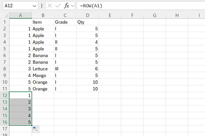
Check the last category sequence in column A, which is A11. In our data, it is 5. We need sequence numbers from 1 to 5.
In cell A12, enter the formula =ROW(A1) and drag it down to A16. This will generate the sequence 1 to 5.
Step 3: Inserting Blank Rows After Each Category
- Select the range A2:D16.
- Click on the Data tab in the ribbon at the top of your Excel Spreadsheet.
- In the Sort & Filter group, click the A->Z button to sort your data in ascending order by the first column in the range.
- After sorting, clear the content in column A.
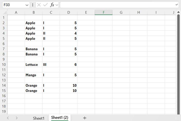
This method will help you add a blank row below each category change in Excel.
Dynamic Array Formula to Add a Blank Row After Each Category Change in Excel
Assuming the source data is the output of an array formula in Excel 365 or other versions of Excel that support dynamic arrays, the helper formula approach described earlier may not work.
Instead, you can use a dynamic array formula to add a blank row after each category change. Based on the sample data, here is the formula:
=DROP(
   REDUCE(
      "", UNIQUE(B2:B11),
      LAMBDA(accu, val,
         IFNA(VSTACK(accu, FILTER(B2:D11, B2:B11=val), ""), "")
      )
   ), 1
)
Insert this formula in cell F2.
In this formula:
- Replace B2:D11 with your source data range.
- Replace B2:B11 with your category range.
This formula is flexible enough to add multiple blank rows. To do this, replace "" immediately after val), with "", "" (for two blank rows), "", "", "" (for three blank rows), and so on.
Formula Explanation
If you’re curious about the logic behind adding blank rows below categories using this dynamic array formula, go through this explanation. If you prefer to skip this part, feel free to do so.
The formula uses the REDUCE function and the syntax is as follows:
REDUCE(initial_value, array, lambda(accumulator, value, function))Where:
intial_value:""(an empty string)array:UNIQUE(B2:B11)(returns the unique categories from the specified range)
The formula uses the following LAMBDA function (a custom unnamed function): LAMBDA(accu, val, IFNA(VSTACK(accu, FILTER(B2:D11, B2:B11=val), ""), ""))
FILTER(B2:D11, B2:B11=val): Filters the source data where the category column matches the current element in the unique category list. Here,valrepresents the current element. The result is stored in the accumulator namedaccu.VSTACK(accu, …, ""): The VSTACK function vertically stacks the accumulator (accu) with the filter result and then adds a blank cell.
REDUCE iterates over each value (val) in the unique category range. For each iteration, it filters the data by category and adds a blank cell below the filtered data. This effectively inserts a blank row below each category, with the first cell empty and the other cells in that row padded with #N/A.
- IFNA: Removes the #N/A errors.
- DROP: Removes the empty row at the top, which is caused by the initial empty cell in the accumulator. This ensures that the result doesn’t have an extra blank row at the top.
This formula allows you to add a blank row below each category using dynamic arrays in Excel.