Highlighting groups with alternating colors can improve readability in Excel. It has another advantage: you can filter every alternate group by applying a filter and selecting ‘Filter by Color’.

Alternating row color is a common practice in spreadsheets. However, sometimes we may want to take it one step further, such as highlighting groups with alternating colors. It’s easy to do without using multiple formulas or helper columns (cells) in Excel.

We have a table with a few electronic items, sorted item-wise, in column A, along with their units and quantities. The items are Laptop, Tablet, Smartphone, Smartwatch, and Headphones.

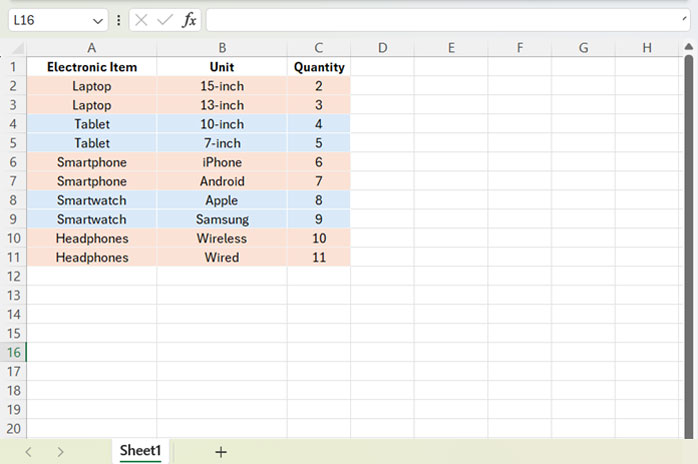
How do we highlight the rows containing “Laptop”, “Smartphone”, and “Headphones”—that means every alternating group—in Excel?

New Rule to Highlight Groups with Alternating Colors in Excel

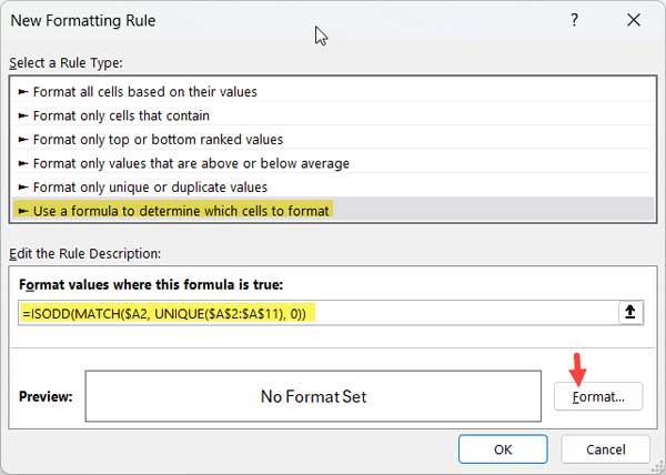
Here is the formula that we will apply within Conditional Formatting to highlight every alternating group with a color:

=ISODD(MATCH($A2, UNIQUE($A$2:$A$11), 0))

Where $A2 represents the very first cell in the column that determines the group, and $A$2:$A$11 is the range of the group.

Before we apply this within Excel’s conditional formatting as a ‘New Rule’, let’s learn what this formula does.

Formula Breakdown

You can skip this part as it is included only for educational purposes.

UNIQUE($A$2:$A$11) – This function returns the unique values from the specified range, removing duplicates:

Laptop
Tablet
Smartphone
Smartwatch
Headphones

MATCH($A2, …, 0) – This function matches the first item in the group among the unique values above and returns its position. For example, it returns 1 for “Laptop” because it is the first item in the unique list.

ISODD(…) – This function returns TRUE if the position is an odd number.

Here is the crux of highlighting groups with alternating colors in Excel. We will apply this formula as a ‘New Rule’ within Conditional Formatting for the range A2:C11. If any cell reference is relative in the formula, it will increment in each row.

In our formula, the search key in the MATCH function is relative by row, which is $A2. It will become $A3, $A4, $A5, …, $A11.

This means the MATCH function matches all values in the group with the unique group values. So for “Laptop,” it will return 1 (TRUE), for “Smartphone,” it will return 3 (TRUE), and for “Headphones,” it will return 5 (TRUE), and those rows will be highlighted.

Highlighting Groups with Alternating Colors in Excel

First, copy the above formula and follow the instructions below:

1. Select the range A2:C11.
2. In the Home tab, within the Styles group, click on Conditional Formatting > New Rule.
3. Select “Use a formula to determine which cells to format.”
4. In the field under “Format values where this formula is true,” paste the copied formula.
   
5. Click the “Format” button to open the Format Cells dialog box.
6. Select a Fill Color you want.
7. Click OK to close the Format Cells dialog box.
8. Click OK again to close the New Formatting Rule dialog box.

This will highlight every other group with the chosen color, leaving an unfilled group between each highlighted group. If you want to highlight those groups with a different color, do as follows:

Follow the above steps 1 to 8 and use the following formula in the formula field:

=ISEVEN(MATCH($A2, UNIQUE($A$2:$A$11), 0))

Resources

• Applying Alternating Colors to Visible Rows in Google Sheets & Excel