Creating hierarchical numbering sequences in an Excel spreadsheet can significantly improve the way you organize and present data.
By utilizing a dynamic array formula, you can establish a clear structure that highlights relationships between main items and their corresponding sub-items.

While we’ve explored similar methods in Google Sheets (see resources at the bottom), it’s important to note that the formulas may differ due to variations in how Excel and Google Sheets handle array outputs within LAMBDA functions.
Purpose of Hierarchical Sequences in Excel
The purpose of hierarchical sequences in Excel is to help users organize and present data in a structured format. This approach enhances:
- Visual Organization: Clearly shows relationships between main items and sub-items, making data easier to read and comprehend.
- Outline Creation: Facilitates the creation of outlines or lists that reflect the hierarchical nature of information, which is useful for project management (e.g., tasks and subtasks), documentation, and reports.
- Improved Navigation: Allows users to quickly identify sections and subsections, enhancing overall document navigability.
- Advanced Level Filtering: Assists in filtering main or sub-tasks based on their hierarchical sequence.
And much more!
Preparing the Input Values
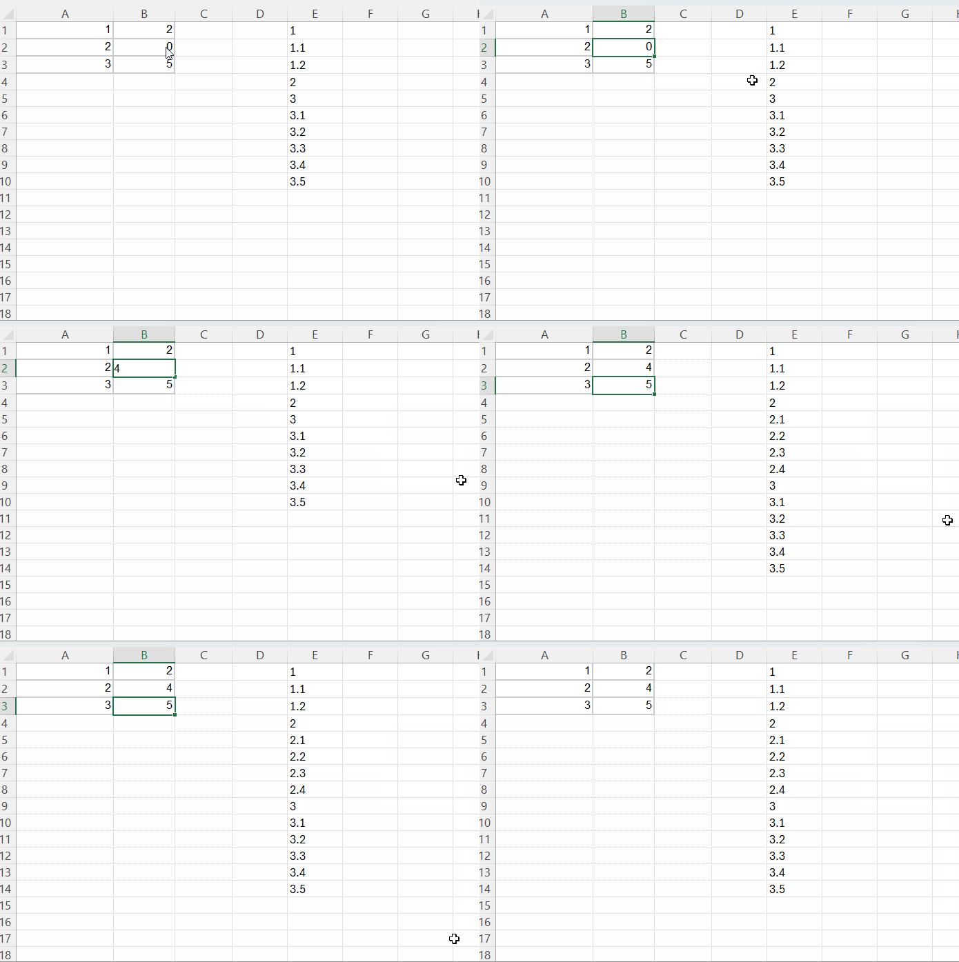
To begin creating hierarchical sequences, you first need to set up your input values. In Column A, enter the main sequence numbers (e.g., 1, 2, 3), and in Column B, specify how many sub-levels you want for each main item.
For example, consider the following setup in cells A1:B3:
| A | B |
| 1 | 2 |
| 2 | 0 |
| 3 | 5 |
Based on this input, Excel will return the following hierarchical numbering sequences:
1
1.1
1.2
2
3
3.1
3.2
3.3
3.4
3.5
This structure effectively shows the main items and their corresponding sub-levels, providing a clear outline.
Formula and Application
To generate these hierarchical sequences, you can utilize the following formula in Column C or any other empty column:
=TOCOL(
   TEXTSPLIT(
      TEXTJOIN("|", TRUE,
         MAP(
            A1:A3, B1:B3,
            LAMBDA(x, y,
               TEXTJOIN("|",TRUE, VSTACK(x,IF(y>0, x&"."&SEQUENCE(y),"")))
            )
         )
      ) ,"|"), 1
)
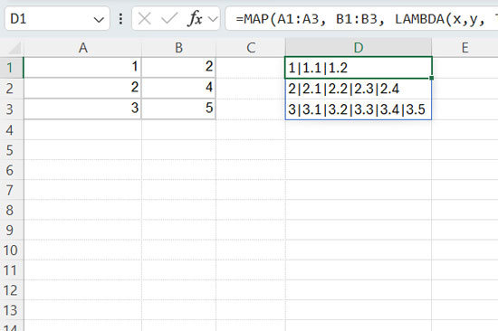
As an example, enter this formula in cell D1. Here, A1:A3 refers to the main sequence, while B1:B3 denotes the number of sub-levels. You can adjust these ranges as per your specific requirements.
Formula Breakdown
For those who are curious about how this formula generates hierarchical sequences, here’s a detailed breakdown of the components:
=SEQUENCE(B1): This function returns a sequence of numbers based on the value in cell B1. If B1 is 2, it produces the numbers 1 and 2.
=IF(B1 > 0, A1 & "." & SEQUENCE(B1), ""): This conditional formula checks if the value in B1 is greater than 0. If so, it combines the value in A1 with a dot and the sequence numbers. For the current setup, if A1 is 1 and B1 is 2, it will yield:
1.1
1.2
VSTACK Function: The VSTACK function is used to vertically stack the main sequence with any sub-level sequences derived from it: =VSTACK(A1, IF(B1 > 0, A1 & "." & SEQUENCE(B1), ""))
1
1.1
1.2
TEXTJOIN: This function concatenates the results, placing a “|” delimiter between each combined value. This step is crucial for preparing the data to be processed by the LAMBDA function: =TEXTJOIN("|", TRUE, VSTACK(A1, IF(B1 > 0, A1 & "." & SEQUENCE(B1), "")))
1|1.1|1.2
LAMBDA Function: The LAMBDA function encapsulates the logic required to process each pair of values in columns A and B: LAMBDA(x, y, TEXTJOIN("|", TRUE, VSTACK(x, IF(y > 0, x & "." & SEQUENCE(y), "")))) Here, x corresponds to the main sequence from Column A, and y corresponds to the number of sub-levels from Column B.
Using the MAP Function: The MAP function applies this LAMBDA function across the arrays in A1:A3 and B1:B3, producing a hierarchical sequence row by row: =MAP(A1:A3, B1:B3, LAMBDA(x, y, TEXTJOIN("|", TRUE, VSTACK(x, IF(y > 0, x & "." & SEQUENCE(y), "")))))

This process generates a flattened string of hierarchical values separated by the “|” delimiter.
Finalizing the Output: The last steps involve joining the strings again and splitting the values using TEXTSPLIT to transform the result into a single-column format with TOCOL: =TEXTJOIN("|", TRUE, MAP(A1:A3, B1:B3, LAMBDA(x,y, TEXTJOIN("|", TRUE, (VSTACK(x, IF(y > 0, x & "." & SEQUENCE(y), "")))))))
1|1.1|1.2|2|2.1|2.2|2.3|2.4|3|3.1|3.2|3.3|3.4|3.5
By executing this entire formula, you create a well-organized set of hierarchical numbering sequences in Excel.


