Hierarchical Number Sorting in Excel with Modern Functions

A hierarchical numbering system in Excel allows you to organize data into a clear, multi-level structure, such as main categories, subcategories, and further subdivisions. However, sorting such numbering can be challenging because the numbers are stored as text. Conventional sorting may not produce the desired result. With the advent of dynamic array functions such as SORT, SORTBY, and TEXTBEFORE, you can now easily perform hierarchical number sorting in Excel.

Formula for Hierarchical Number Sorting

This formula enables you to sort multi-level (outline) numbers with any number of levels. Here’s the formula:

=LET(
   outlinen, A2:A15, 
   delimiter, ".", 
   n, MAX(LEN(outlinen)-LEN(SUBSTITUTE(outlinen, ".", ""))+1), 
   split, TEXTBEFORE(TEXTAFTER(delimiter&outlinen&delimiter, delimiter, SEQUENCE(1, n)), delimiter, 1), 
   splitF, N(IFERROR(IFERROR(split*1, split), "")), 
   seqR, SEQUENCE(ROWS(outlinen)), 
   sortIndex, SEQUENCE(1, COLUMNS(splitF), 2), 
   sortOrder, SEQUENCE(1, COLUMNS(splitF), 1, 0), 
   srt, CHOOSECOLS(SORT(HSTACK(seqR, splitF), sortIndex, sortOrder), 1), 
   ids, XMATCH(seqR, srt), 
   SORTBY(HSTACK(A2:A15&""), ids, 1)
)

When using this formula, replace A2:A15 with the reference for the column containing the hierarchical numbers to sort. If additional columns need sorting, include them in the HSTACK. For instance:

Replace HSTACK(A2:A15&"") with HSTACK(A2:A15&"", B2:B15) for two columns.
Replace it with HSTACK(A2:A15&"", B2:C15) for three columns.

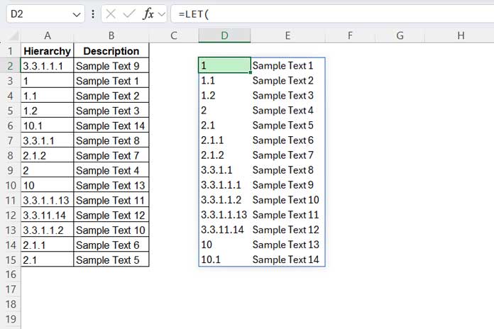
Example of Hierarchical Number Sorting in Excel

In the following example, Column A contains hierarchical numbering, and Column B contains descriptions.

Here’s how to sort this data:

Select A2:A15.
Navigate to the Home tab and select Text from the drop-down in the Number group. This formats the hierarchical numbers as text. Numbers like 1, 2, 3, which are typically numeric, will also be converted to text.
Enter the formula in D2:

=LET(
   outlinen, A2:A15, 
   delimiter, ".", 
   n, MAX(LEN(outlinen)-LEN(SUBSTITUTE(outlinen, ".", ""))+1), 
   split, TEXTBEFORE(TEXTAFTER(delimiter&outlinen&delimiter, delimiter, SEQUENCE(1, n)), delimiter, 1), 
   splitF, N(IFERROR(IFERROR(split*1, split), "")), 
   seqR, SEQUENCE(ROWS(outlinen)), 
   sortIndex, SEQUENCE(1, COLUMNS(splitF), 2), 
   sortOrder, SEQUENCE(1, COLUMNS(splitF), 1, 0), 
   srt, CHOOSECOLS(SORT(HSTACK(seqR, splitF), sortIndex, sortOrder), 1), 
   ids, XMATCH(seqR, srt), 
   SORTBY(HSTACK(A2:A15&"", B2:B15), ids, 1)
)

This formula will sort the data in A2:B15 by arranging the hierarchical numbers in ascending order.

The Logic Behind Sorting Hierarchical Numbers in Excel

In hierarchical numbering, each individual number represents different levels of hierarchy and is separated by a period. For example, consider the number 1.1.2:

1: The top-level or primary number, often representing the main category or section.
1: The second-level or subsection, nested under the first number.
2: The third-level or sub-subsection, further nested under the second level.

When performing hierarchical number sorting, we first split the numbers into individual columns and sort each column in ascending order dynamically. You do not need to specify each column for sorting manually. Fortunately, Excel’s SORT function supports arrays in sort_index (the columns to sort) and sort_order (the order to sort).

Note: The Google Sheets SORT function does not support this. Instead, you can use the QUERY sorting feature in Google Sheets. See the Resources section for a relevant tutorial titled "multi-level numbers."

Returning to the logic: during sorting, we include a sequence number column with the sort range, which we do not sort. We extract this column and match the sequence numbers of the hierarchical numbers. These relative positions are then used to sort the hierarchical numbering using the SORTBY function.

Formula Explanation

The formula has several components. Let’s break it down for clarity:

Basic Components

outlinen: Refers to the hierarchical sorting range (A2:A15).
delimiter: Specifies the delimiter used to separate levels (a period “.”).

Splitting Components

n: Calculates the maximum number of levels in the hierarchy.
split: Splits the hierarchical numbers into multiple columns.
splitF: Converts text-formatted numbers in split result to numeric values and replaces errors or empty cells with blanks.

Sorting Components

seqR: Generates a sequence number for each row.
sortIndex: Determines the column indices to sort by.
sortOrder: Specifies the sort order for each column.
srt: Sorts the split numbers in ascending order and extracts the corresponding sequence numbers.

Final Sorting

ids: Matches the original sequence numbers to their sorted positions.
SORTBY: Sorts the combined range (HSTACK) based on the relative positions (ids).

By using the above formula, you can efficiently perform hierarchical number sorting in Excel for multi-level data. Whether you’re dealing with nested outlines or multi-level lists, this method simplifies the sorting process using Excel’s modern functions.