


")


")

")
")
 in Excel & Google Sheets")


You can find missing dates in a list in Excel using either a VLOOKUP formula with a helper column or a dynamic array formula. We’ll explore both approaches since the dynamic array formula won’t work in older Excel versions.
For the following examples, consider a small date range in A2:A5:
| 01-01-2024 |
| 02-01-2024 |
| 05-01-2024 |
| 08-01-2024 |
The missing dates in this range are:
| 03-01-2024 |
| 04-01-2024 |
| 06-01-2024 |
| 07-01-2024 |
Find Missing Dates Using Helper Column and VLOOKUP in Excel
To get started, let’s use a helper column and VLOOKUP to identify the missing dates.
In cell B2, enter the following formula to find the minimum date in the range A2:A5:
=MIN(A2:A5)This will return the minimum date from your range.
In cell B3, enter the following formula and copy it down until it returns a hyphen (“-“):
=IFERROR(IF(B2+1<=MAX($A$2:$A$5), B2+1, "-"),"")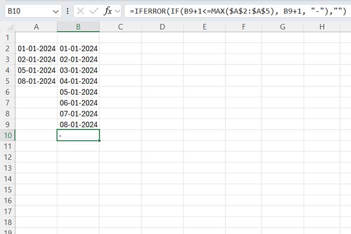
This formula creates a list of sequential dates starting from the minimum date, incrementing by 1 each time, until it reaches the maximum date in your range. It will display a hyphen (“-“) if the date exceeds the range.
The result of the formula will be date values in Excel. To ensure the dates are formatted correctly, select the results in column B, navigate to the Home tab, and choose Short Date from the Number group.
Now, in cell C2, enter the following VLOOKUP formula and drag it down:
=IF(IFERROR(VLOOKUP(B2, $A$2:$A$5, 1, 0),0),"-", "Missing")This formula checks if each date in column B is present in the original list of dates in column A. If it finds a match, it returns a hyphen (“-“); if it doesn’t, it returns the text “Missing.”
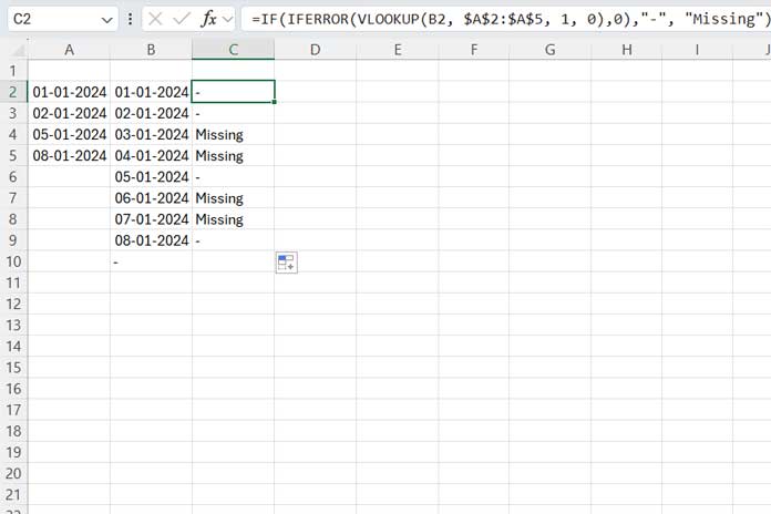
This method is a classic way to find missing dates in Excel using a helper column with VLOOKUP.
Find Missing Dates Using a Dynamic Array Formula in Excel
If you’re using a version of Excel that supports dynamic arrays, the process becomes much simpler.
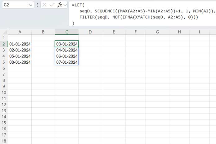
To find missing dates in the range A2:A5, use this formula:
=LET(
   seqD, SEQUENCE((MAX(A2:A5)-MIN(A2:A5))+1, 1, MIN(A2)),
   FILTER(seqD, NOT(IFNA(XMATCH(seqD, A2:A5), 0)))
)Note: You should format the result as Short Date or Long Date from the Number group on the Home tab.
Here’s how the formula works:
The SEQUENCE((MAX(A2:A5)-MIN(A2:A5))+1, 1, MIN(A2)) part generates a sequence of dates starting from the minimum date in the range and continuing to the maximum date.
- The
(MAX(A2:A5)-MIN(A2:A5))+1calculates how many rows are needed to cover the full range of dates. The1indicates a single-column result, andMIN(A2)sets the starting point for the sequence.
The FILTER(seqD, NOT(IFNA(XMATCH(seqD, A2:A5), 0))) part filters the sequence of dates.
XMATCH(seqD, A2:A5)compares each date in the sequence to the dates in your original range. If a date is found, it returns the relative position of that date; if not, it returns an error.- The IFNA function replaces those errors with 0.
- The NOT function converts 0 into TRUE (indicating the date is missing) and valid positions into FALSE.
- The FILTER function then returns only the dates that are missing from the list, i.e., when the condition is TRUE.
This method is much more efficient if you have a newer version of Excel that supports dynamic arrays.
Conclusion
Both methods will help you identify missing dates in Excel, with the VLOOKUP approach working in older versions and the dynamic array formula being faster and more elegant for newer versions. Depending on your Excel version, choose the method that best suits your needs.