
 in Google Sheets")

")


")


")


Finding the last used column in Excel is a common need, but most available methods simply count the number of columns in a range. This can be misleading when the rightmost columns are empty.
For example, if your data expands across columns, and your range is A1:Z100, but the actual data only extends to column E, counting columns would return 26 instead of the correct value, 5.
In this tutorial, we’ll use a dynamic Excel formula that accurately identifies the last non-empty column in a given range. Instead of returning the total column count, this method ensures that only columns containing data are considered.
This formula does not require every row in a column to be filled. Even a single non-empty cell in a column will count.
How It Works
Our approach leverages the TRIMRANGE function, which is currently available in Excel 365. This makes the formula both efficient and adaptable, ensuring accurate results even as your data structure changes.
Formula to Find the Last Column with Data in Excel
1. Get the Last Column Number with Data
=MAX(COLUMN(TRIMRANGE(range, 3, 3)))Replace range with the actual data range, e.g., Sheet1!A1:Z100.
Example Output: If column G is the last non-empty column, the formula will return 7.
2. Get the Column Letter of the Last Used Column
=REGEXEXTRACT(ADDRESS(1, MAX(COLUMN(TRIMRANGE(range, 3, 3)))), "[A-Z]+")Again, replace range with the actual data range.
Example Output: If the last used column is G, the formula will return "G".
Sample Data
The sample data is currently in B2:E8, but it will gradually expand up to column Z. So, we will use B2:Z8 as the range, and the sheet name is Sheet1.
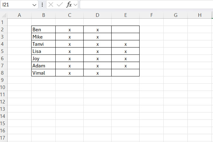
Here, the last column with data is column E, so the formulas will return:
- Column number:
5 - Column letter:
"E"
Example Usage
1. Get the Last Column Number with Data in a Dynamic Range
=MAX(COLUMN(TRIMRANGE(Sheet1!B2:Z8, 3, 3)))Where to enter the formula?
Place this formula in any cell outside the range (or in another worksheet). It will return the correct last used column number.
The formula is dynamic – if you enter new data, the column number will update automatically.
2. Get the Column Letter of the Last Used Column
=REGEXEXTRACT(ADDRESS(1, MAX(COLUMN(TRIMRANGE(Sheet1!B2:Z8, 3, 3)))), "[A-Z]+")Example Output: "E" if column E is the last non-empty column.
Formula Breakdown
Step 1: Trim Empty Columns
TRIMRANGE(Sheet1!B2:Z8, 3, 3)This function removes empty columns and rows from the range dynamically.
Step 2: Find the Column Numbers of Non-Empty Columns
COLUMN(TRIMRANGE(Sheet1!B2:Z8, 3, 3))This returns an array of column numbers that contain data.
Step 3: Find the Column Number of the Last Used Column
MAX(COLUMN(TRIMRANGE(Sheet1!B2:Z8, 3, 3)))The MAX function returns the highest column number from the array in the previous step, representing the last used column.
Step 4: Convert the Column Number to a Letter
ADDRESS(1, MAX(...))This converts the column number into an Excel cell reference, such as "E1".
REGEXEXTRACT(..., "[A-Z]+")The REGEXEXTRACT function extracts only the column letter from the cell reference, giving the final result.
FAQs
What happens if the cell range is empty?
If the range has no data, the formula returns #REF!.
Fix: Wrap the formula with IFERROR:
=IFERROR(formula_here, "")Does this formula work in older Excel versions?
No. This formula requires Excel 365, as it relies on TRIMRANGE, LET, and REGEXEXTRACT.
Final Thoughts
This method ensures that only columns with data are considered when finding the last used column in Excel. Unlike traditional methods that just count columns, this approach dynamically adapts to changes in your data.
Try the formulas above and let me know if you have any questions!
Related Resources
More Excel & Google Sheets Tutorials: