You can use the REGEXEXTRACT or REGEXREPLACE functions to easily extract numbers from text in Excel. The choice of function depends on whether your text contains multiple numbers or just one.
Many applications import data into Excel, and when working with such data, you may encounter numbers embedded in text strings.
For example:
- Invoice numbers such as “Invoice #1564”
- Product IDs such as “AI123456”
- Amounts such as “USD 1500.00”
- Text strings such as “January sales are worth 10.5 million US dollars, and February sales are worth 12.5 million US dollars”
You might want to extract numbers from the left, right, a specific position, or all numbers from a text string in Excel. Depending on the scenario, you can use REGEXEXTRACT, REGEXREPLACE, or a combination of functions like REGEXREPLACE, TEXTSPLIT, and CHOOSECOLS.
Let’s look at examples for all these scenarios below.
Regex to Extract Numbers from Left of Text in Excel
Assume the text in cell A1 is “Invoice #1564”. The following REGEXEXTRACT formula will return 1564:
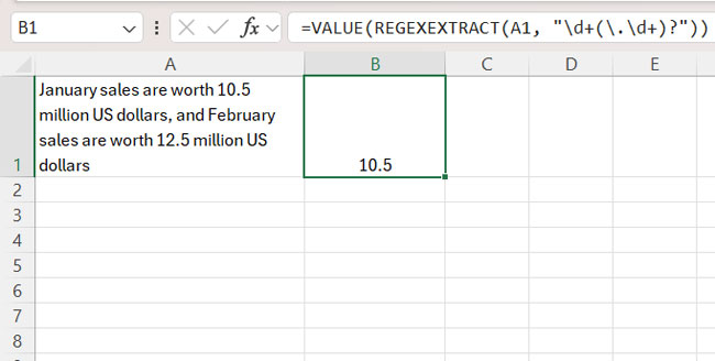
=VALUE(REGEXEXTRACT(A1, "\d+(\.\d+)?"))If the text is “January sales are worth 10.5 million US dollars, and February sales are worth 12.5 million US dollars”, the output will be the first number in the string, which is 10.5.

This formula can extract both decimal numbers and integers from the text. If there are multiple numbers, it will extract the first one.
Regarding the regex pattern, \d+ matches one or more digits, and (\.\d+)? optionally matches a decimal point followed by one or more digits. This ensures the formula extracts the first number, including decimals if present.
Regex to Extract Numbers from Right of Text in Excel
The following formula will extract the last number present in the text string in Excel:
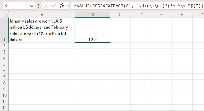
=VALUE(REGEXEXTRACT(A1, "\d+(\.\d+)?(?=[^\d]*$)"))If the text contains just one number, it will return that number. If there are multiple numbers, it will return the last number. Similar to the first example, this formula is also capable of extracting both decimals and integers.

The first part of the regex pattern, \d+(\.\d+)?, is the same as in our first formula, used to extract the first number, including decimals if present. The last part, (?=[^\d]*$), is a positive lookahead that ensures the number being matched is followed by non-digit characters (or no characters at all), meaning it’s the last number in the string.
How to Extract All Numbers from Text in Excel
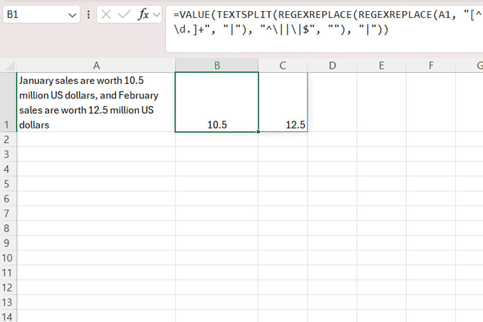
When you have multiple numbers in a string and want to extract all numbers from text in Excel into individual cells in a row, you can use the following combination formula:
=VALUE(TEXTSPLIT(REGEXREPLACE(REGEXREPLACE(A1, "[^\d.]+", "|"), "^\||\|$", ""), "|"))
In this formula:
- The inner regex replaces all non-numeric and non-period characters (one or more times, indicated by
+) with a single pipe (|). - The outer regex replaces any leading or trailing pipe characters (
|) with an empty string, i.e.,"". - The TEXTSPLIT function splits the result at the pipe character (
|), separating the numbers.
Extracting Specific Numbers from Text
You can use the formula above to extract all numbers from text in Excel. To extract specific numbers based on their position, wrap the formula with the CHOOSECOLS function.
The syntax is: =CHOOSECOLS(…, n)
For example, the following formula will return 1200 if the string in cell A1 is:
“The total cost of the project is $3500, with an initial deposit of $500 and additional expenses of $1200. The remaining balance is $1800.”
=CHOOSECOLS(VALUE(TEXTSPLIT(REGEXREPLACE(REGEXREPLACE(A1, "[^\d.]+", "|"), "^\||\|$", ""), "|")), 3)The Role of VALUE in the Formulas
We used the VALUE function with all formulas to convert the text-formatted numbers returned by the formula into actual numbers so that we can use them in calculations.
It also plays an important role in formulas that use REGEXREPLACE. For example:
If a string ends with a number followed by a period, such as “Received $100.”, the formula will return “100.”. Using the VALUE function ensures that it returns just 100 without the period.


