You can use the following formula to extract the last N non-blank rows in Excel:

=TAKE(FILTER(range, BYROW(range, LAMBDA(row, COUNTA(row)>0))), -N)

where:

• range – The range to filter.
• N – The number of last non-blank rows you want to extract.

Introduction

Extracting the last N non-blank rows from a dataset is especially useful when dealing with dynamic data where blank rows may appear in between. Additionally, if you reference a large range to accommodate future entries, there will definitely be blank rows at the end.

Extracting the last N non-blank rows has several benefits, such as:

• Analyzing the most recent entries while ignoring blanks.
• Creating a dynamic report that updates as new data is added.
• Extracting the latest transactions, sales, or stock updates from a dataset.

Example

Assume your data is in the range A1:C1000, but actual data is present only up to row 31 (A1:C31), with some blank rows in between. If you want to extract the last 10 non-blank rows, you can use the following formula:

=TAKE(FILTER(A1:C1000, BYROW(A1:C1000, LAMBDA(row, COUNTA(row)>0))), -10)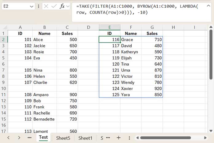

How This Formula Works

• BYROW(A1:C1000, LAMBDA(row, COUNTA(row)>0)): Checks each row to see if it has at least one non-blank cell.
  • The COUNTA function counts the values in the current row.
  • >0 ensures that the function returns TRUE for non-blank rows and FALSE for blank rows.
  • BYROW applies this check to each row in the range.
• FILTER(A1:C1000, … ) : Keeps only the non-blank rows from the dataset.
  • It filters the rows where BYROW returns TRUE.
• TAKE( … , -10 ): Extracts the last 10 rows from the filtered dataset.

Additional Tip: Extract N Rows from the Last Non-Blank Row to the Top

If you just want to remove empty rows from the bottom and extract 10 rows from the last non-blank row, you can use a combination of TRIMRANGE and TAKE as follows:

=TAKE(TRIMRANGE(A1:C1000), -10)

• The TRIMRANGE function removes empty rows from the bottom.
• The TAKE function extracts the last 10 rows from this trimmed range.

This formula is more resource-friendly as it doesn’t use the BYROW Lambda function.

Resources

• How to Retrieve the Last Record in Each Group in Excel
• Find the Last Used Row Number in Excel
• Find the Last Used Row’s Last Value Address in Excel
• Hyperlink to Jump to the Last Used Row in Excel