This tutorial demonstrates how to calculate the running total by month in a range or table in an Excel spreadsheet.
To calculate the running total by month in a range, you can use a dynamic array formula if you are using Excel 365, or a drag-down formula in earlier versions.
I would prefer the table approach for this calculation, as the dynamic array formula uses a Lambda function that may not perform optimally with extensive datasets.
Running Total By Month in a Table in Excel
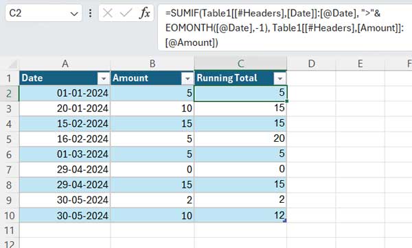
My table in Excel contains the labels “Date” in cell A1, “Amount” in cell B1, and “Running Total” in cell C1.
Cells A2:A10 contain dates, B2:B10 contain amounts, and C2:C10 is currently empty where we will generate the running total by month.
First, you should sort this table by the dates in ascending order. To do so, click the drop-down in cell A1 and select “Sort Oldest to Newest”.

In cell C2, enter the following formula to generate the running total by month in the range C2:C10:
=SUMIF(Table1[[#Headers],[Date]]:[@Date], ">"&EOMONTH([@Date],-1), Table1[[#Headers],[Amount]]:[@Amount])Make changes if your table contains different field labels.
For example, if your table has the label “Sales Amount” instead of “Amount” in cell B1, replace “Amount” in the formula with “Sales Amount”.
Also, if your table name is different, replace “Table1” with the actual name of your table.
To find the current table name in Excel, follow these steps:
- In a blank cell outside the table range, enter the formula
=A1(assuming A1 is any cell within the first or second row of the table). - Press Enter.
- Navigate to the cell where you entered the formula and look at the formula displayed in the formula bar.
You will find the name of the table displayed in the formula.
Formula Logic
The formula utilizes the SUMIF function in Excel to sum values in a range based on a provided condition in another range.
Syntax: =SUMIF(range, criteria, sum_range)
In each row, the formula tests whether the dates in the range, from the header to the current row, are greater than the end of the month date of the previous month, which is derived from the date in the current row.
It then sums up the values in column B to the current row if the test evaluates to TRUE.
Running Total By Month in a Range in Excel
You can consider the following formulas in a sorted range if you prefer using a range instead of a table.
Basic Drag-Down Formula
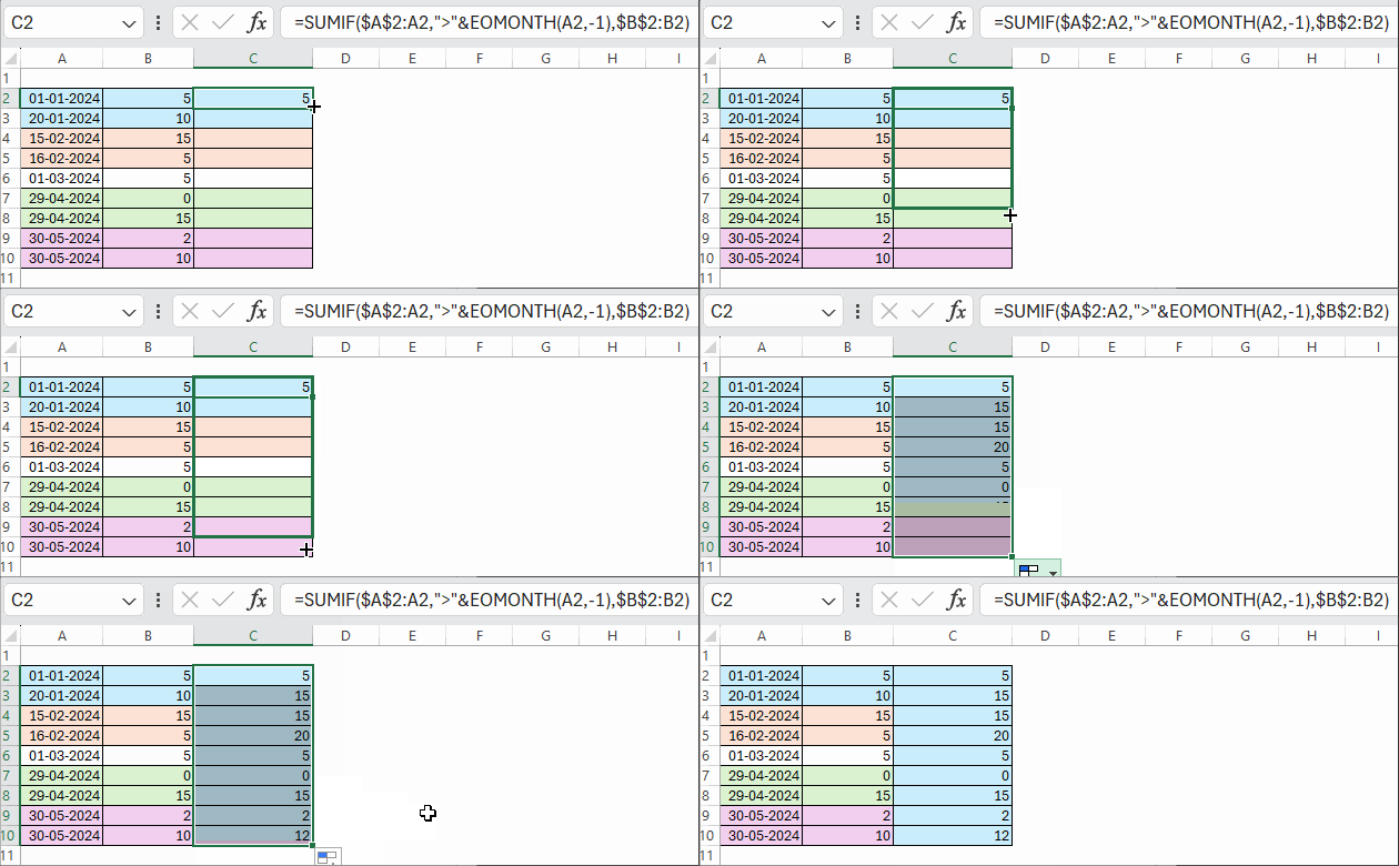
We have dates in A2:A10 and amounts in B2:B10. To get the running total by month in C2:C10, enter the following SUMIF formula in cell C2:
=SUMIF($A$2:A2,">"&EOMONTH(A2,-1),$B$2:B2)Navigate to cell C2, if not already there, and drag the fill handle down until C10.

As you drag down, the range $A$2:A2 becomes $A$2:A3, $A$2:A4, and so forth, adjusting accordingly for each row. The same applies to the sum_range.
This formula follows the same logic as the one used in the table to calculate the monthly running total.
It sums the amounts from the first row to the current row in each row by applying a condition.
The condition checks whether the dates up to the current row are greater than the end-of-the-month date of the previous month. The end-of-the-month date of the previous month is derived from the date in the current row.
If the condition evaluates to TRUE, the formula sums the amounts for those rows.
Dynamic Array Formula
If you’re using Excel 365 or a version that supports the MAP function and dynamic arrays, there’s no need for the drag-down formula mentioned earlier.
Insert the following formula in cell C2:
=MAP(A2:A10, B2:B10, LAMBDA(dates, amount,
   SUMIF($A$2:dates, ">"&EOMONTH(dates, -1), $B$2:amount)
))
This formula will automatically spill down the running total by month in your data range in Excel.
Here’s how it works:
We use the MAP function to iterate over each row in the arrays A2:A10 and B2:B10.
The corresponding defined names are “dates” and “amount”. So in the SUMIF formula, we use $A$2:dates and $B$2:amount instead of $A$2:A2 and $B$2:B2.
Conclusion
All the running total formulas mentioned in this tutorial are for summing by month and year, not just by month. This is because we haven’t used the month number; instead, we used dates for the evaluation.
So if your data is spread across different years, you can use the same formulas without having issues.
Before you input the formula, please ensure you’ve sorted your data by date in ascending order.


