With the help of the LAMBDA function, you can create both named and unnamed custom functions in Excel (not supported in all versions).
Named functions are standalone and can be used throughout the workbook like native Excel functions. Unnamed functions are specific to LAMBDA helper functions such as BYROW, BYCOL, and REDUCE, where they are defined.
The syntax of the Excel LAMBDA function is as follows:
=LAMBDA([parameter1, parameter2, …,] calculation) parameter1: The name used inside the calculation. When using the custom function created by LAMBDA, you can pass a value to this name, such as a cell reference, string, or number.parameter2, …: Additional names, if any.calculation: The formula to be calculated and return the result of the function. It uses names declared in the previous parameters.
Note: You can enter up to 253 parameters, but you’re unlikely to use that many.
How to Create Your First LAMBDA Function in Excel
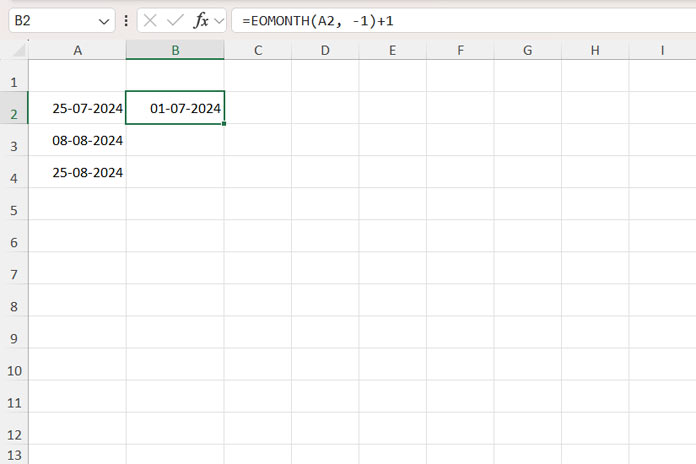
Assume you want to find the beginning of the month date for the date in cell A2. You usually use the following formula in Excel:
=EOMONTH(A2, -1)+1
Here’s how to create a custom unnamed LAMBDA function that performs the same calculation:
=LAMBDA(cell_ref, EOMONTH(cell_ref, -1)+1)In this example, cell_ref is the parameter, and EOMONTH(cell_ref, -1) + 1 is the calculation.
You can pass a cell to this parameter when you use it as a named function or within helper functions.
Before naming or using the function, you can test whether this unnamed function works properly by directly passing the cell reference as follows:
=LAMBDA(cell_ref, EOMONTH(cell_ref, -1)+1)(A2)The last part (A2) is called the function call.
Note: The output may appear as a date value. If so, navigate to the result cell, click the Home tab, and select either Short Date or Long Date from the drop-down menu in the Number group.
Using Unnamed LAMBDA Functions in Excel
You have created your first unnamed LAMBDA function in Excel. How do you use it?
You can use unnamed LAMBDA functions with the following core LAMBDA helper functions:
- BYROW: Applies a LAMBDA function to each row of an array.
- BYCOL: Applies a LAMBDA function to each column of an array.
- MAP: Applies a LAMBDA function to each element of an array.
- REDUCE: Combines elements of an array into a single value using a LAMBDA function.
- SCAN: Similar to REDUCE, but returns an array of intermediate results.
- MAKEARRAY: Creates a calculated array of specified dimensions using a LAMBDA function.
- ISOMITTED: Checks if a LAMBDA argument is omitted and returns TRUE or FALSE.
In this example, we want to pass a cell to the LAMBDA function, such as A2.
To do this, use the MAP function:
=MAP(A2, LAMBDA(cell_ref, EOMONTH(cell_ref, -1)+1))It will return the first day of the month for the date in cell A2.
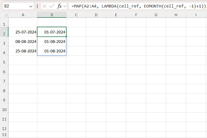
The MAP function applies the custom LAMBDA function to each element of an array. For example, if you specify A2:A4, it returns the beginning of the month date for each value in the array:
=MAP(A2:A4, LAMBDA(cell_ref, EOMONTH(cell_ref, -1)+1))
That’s how to create and use an unnamed LAMBDA function in Excel.
Naming and Reusing Custom Functions with LAMBDA in Excel
Above, we have seen how to create a LAMBDA function and use it within a helper function. Here’s how to name it:

- Click the Formulas tab.
- In the Defined Names group, click Name Manager.
- Click New.
- In the Name field, enter your custom function name, for example,
BOMONTH. - In the Scope field, select where you want the custom function to be available. Choose Workbook.
- In the Refers to field, enter the LAMBDA function, e.g.,
=LAMBDA(cell_ref, EOMONTH(cell_ref, -1) + 1). - Click OK and close the Name Manager.
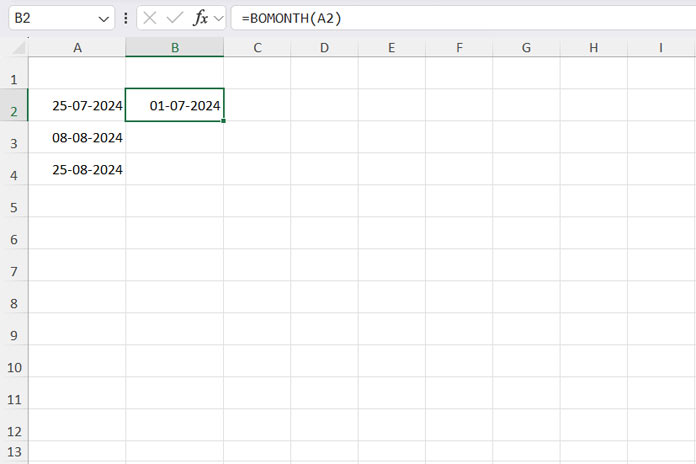
Now you can use the custom-named function to get the beginning of the month date in any cell in the same workbook:
=BOMONTH(A2)
=BOMONTH(Sheet10!A2)
Additional Points
When naming LAMBDA functions and parameters, avoid using names that conflict with Excel’s built-in function names.
Excel requires function names to be a single, continuous string of characters (a maximum of 255 characters) without any spaces or special symbols, except underscores. You can use numbers, but the name cannot start with a number.
Use descriptive names for functions; for example, BOMONTH function represents the beginning of the month. When naming parameters, you can use start_Date or startDate to represent the start date.
Resources
The examples provided in the following resources demonstrate the versatility and power of LAMBDA functions in Excel.


