You can utilize functions like ROW or SEQUENCE in Excel to create a custom descending sequence list.
For Microsoft 365 users, dynamic array formulas based on these functions are available. Otherwise, you can resort to the ROW function.
Mastering this technique empowers you to easily generate lists of descending sequence numbers or dates in Excel.
Creating a Custom Descending Sequence List of Numbers in Excel
If you happen to be using older versions of Excel, you may find this approach helpful.
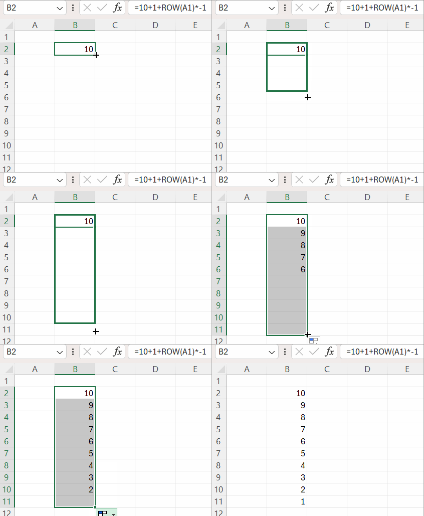
The following formula will return the decremental sequence from 10. Enter it in any cell and drag it down until the formula returns 1:
=10+1+ROW(A1)*-1
Where:
- 10: starting value
- -1: step value
- 1: adjustment value (to ensure the sequence starts at 10, not at 9)
If you want the sequence decreasing by increments of 0.5 from 10 to 0.5, replace the step value in the above formula with -0.5 and the adjustment value to 0.5. The formula will be:
=10+0.5+ROW(A1)*-0.5In the above formulas, change the starting value from 10 to the number of your choice, such as 100, 1000, etc. You will get a negative sequence if you specify -1 as the starting value.
Dynamic Array Formulas for Decremental Sequence in Excel
If you are using Excel in Microsoft 365, there are two options for creating a custom descending sequence list using the ROW and SEQUENCE functions.
Among them, I prefer SEQUENCE due to its simplicity and also because it’s the dedicated function for such calculations. Here they are:
ROW:
=10+1+ROW(A1:A10)*-1This will generate a list of descending sequence numbers from 10 to 1.
Where:
- 10: starting value
- -1: step value
- 1: adjustment value (to ensure the sequence starts at 10, not at 9)
- A10: number of rows.
To create a custom descending sequence decreasing by increments of 0.5 from 10 to 0.5, use the following formula:
=10+0.5+ROW(A1:A20)*-0.5Where:
- 10: starting value
- -0.5: step value
- 0.5: adjustment value (to ensure the sequence starts at 10, not at 9.5)
- A20: number of rows.
SEQUENCE:
To generate a sequence list in descending order, specify -1 as the step value in the SEQUENCE function in Excel.
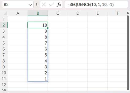
=SEQUENCE(10, 1, 10, -1)This Excel formula follows the syntax SEQUENCE(rows, [columns], [start], [step]).

The above formula will return the numbers from 10 to 1.
To return 10 to 0.5, use the below formula:
=SEQUENCE(20, 1, 10, -0.5)Creating a Custom Descending Sequence List of Dates in Excel
If you know how to create a custom descending sequence of numbers, then converting that to return decrementing sequential dates is quite simple.
You just need to replace the “start” value with a date value in the DATE function syntax DATE(year, month, day).
Examples:
=DATE(2024, 1, 31)+1+ROW(A1)*-1Enter this formula in any cell and drag it down to get the date sequence in descending order from 31/01/2024, 29/01/2024, and so forth.
Don’t forget to format the results to short or long dates by clicking the drop-down within the Numbers group in the Home tab.
Here are the dynamic array formulas:
ROW:
=DATE(2024, 1, 31)+1+ROW(A1:A10)*-1Where:
- DATE(2024, 1, 31): starting value
- -1: step value
- 1: adjustment value (to ensure the sequence starts at DATE(2024, 1, 31), not at DATE(2024, 1, 30))
- A10: number of rows.
SEQUENCE:
=SEQUENCE(10, 1, DATE(2024, 1, 31), -1) // as per SEQUENCE(rows, [columns], [start], [step])Note: You can replace DATE(2024, 1, 31) with TODAY() to get a descending sequence starting from today’s date.
Resources
Here are a few dynamic array formulas in Excel:


