 in Google Sheets")

")

")


")


")


 in supported versions.)
To custom sort in Excel, we can use the SORT command or a dynamic array formula (SORTBY + MATCH combination) in supported versions.
SORTBY is useful if the sort order column is not part of the data table (a distant column) or if you don’t want to alter the original data.
The purpose of custom sorting in Excel is to arrange the data table based on priorities, which could be the status of tasks, sales orders, etc. In some cases, we will use it to sort by month names, weekdays, quarters, or other sequential text-based orders.
In the following example, we have a two-column dataset with task names in one column and their respective statuses in another column.
Sample Data (A1:B12):
| Task | Status |
| Drawing Approval | Completed |
| Material Procurement | In-progress |
| Supply at site | In-progress |
| Excavation | Completed |
| Structural work | Completed |
| Cable Laying | In-progress |
| End Termination | In-progress |
| Cable Jointing | In-progress |
| Backfilling | Pending |
| Testing | Pending |
| Commissioning | Pending |
I want to sort this data based on the statuses in cells B2:B12 in the order “Completed,” “In-progress,” and “Pending.”
Custom Sort Using SORT Command in Excel
You can follow the steps below to sort the above data using the SORT command in a custom order, rather than alphabetically.
Select the data range A1:B12 as per our example.
Click on the “Data” menu and in the “Sort & Filter” group, click on “SORT.”
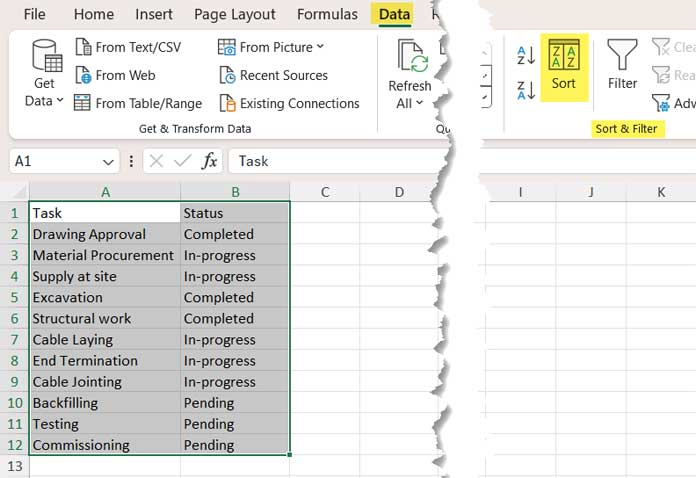
Check “My data has headers.”
Select the column to sort by, which is “Status” in this case.
Choose “Cell values” in the “Sort On” option, as we want to perform the custom sort based on cell values, not on cell color, font color, or conditional formatting icon.
Select “Custom list” in the “Order” section.
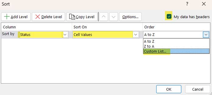
This will open the Custom Lists dialog box, which contains pre-filled custom lists such as weekdays, months, and hierarchy or ranking (“Diamond, Platinum, Gold, Silver”).
We need to create a new list for the custom sort order as per our sample data.
To do this, click on “NEW LIST” and enter “Completed”, “In-progress”, and “Pending”. You can enter one value and hit enter, then another, and so on, or enter them comma-separated.
(Alternatively, you can import a list from within a range in your spreadsheet. We will cover that tip once we complete the custom sort).
Once entered the strings, click “Add” and then “OK.”
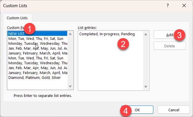
This will close the Custom Lists dialog box. Then click “OK” again to close the Sort dialog box.
This is the simplest way to perform a custom sort in Excel.
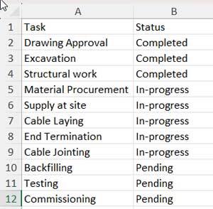
Custom Sort Output:
Importing List Entries for Custom Lists
In our example, we have only three list entries: Completed, In-progress, and Pending. If you have many, you can import them from your spreadsheet.
To do that, follow the steps below:
- Enter the list of entries in your spreadsheet. For example, “Completed,” “In-progress,” and “Pending” in cells D1, D2, and D3 respectively.
- Select cells D1:D3.
- Click on “File” > “Options.” Then, click “Advanced” and scroll down to “General” options.
- Click “Edit Custom Lists,” which will open the Custom Lists dialog box.
- Click “Import.”
Note: The list in cells D1:D3 must not be the result of a formula.
Custom Sort Using a Formula in Excel
If you prefer not to alter your original data, you can use a formula to perform custom sorting in Excel. For this, we can utilize the SORTBY function in combination with MATCH.
Please note that this method may not work in all versions of Excel, as it requires dynamic array functionality and the availability of the SORTBY function.
Generic Formula:
=SORTBY(data, MATCH(column, list_entries, FALSE), TRUE)Where:
data– the data table to sort, excluding the header rowcolumn– the column to sort by in the data tablelist_entries– the custom sort order list
Given our sample data in A1:B12 and the list entries present in cells D1:D3 (“Completed,” “In-progress,” and “Pending”), we can use the following formula to sort by custom list in Excel:
=SORTBY(A2:B12, MATCH(B2:B12, D1:D3, FALSE), TRUE)