


To calculate the running count of values in a list, we can use COUNTIF with or without dynamic array functionality in Excel.
In a sorted or unsorted list, the first occurrence of a value is numbered 1, the second occurrence is numbered 2, and so on. This applies to all the values in the list.
The benefits of using a running count in Excel include:
- Trend and Pattern Identification: Running counts help identify trends and patterns by showing how often specific values occur in a data.
- Conditional Analysis: Running counts can be used in combination with other Excel functions such as FILTER and SUMIFS, enabling conditional analysis based on specific criteria.
- Versatility in Applications: Running counts can be applied in various scenarios, from inventory management to sales tracking, offering flexibility in data analysis.
Running Count of Occurrences Using COUNTIF in Excel
Let’s consider t-shirt colors red, blue, and green in the range C3:C12. These colors occur multiple times in the list.
Insert the following Excel COUNTIF formula in cell D3 and drag it down until D12:
=COUNTIF($C$3:C3, C3)
This will return the running count of occurrences of values, such as t-shirt colors, in the list.
How does this formula work?
When we drag the formula down, the range, i.e., $C$3:C3, becomes $C$3:C4, $C$3:C5, $C$3:C6, and so on. Similarly, the criterion becomes C3, C4, C5, C6, and so on.
So, the formula returns the count of occurrences of the criterion up to the current row, as the range is not the whole range but up to the current row only.
Running Count of Occurrences Using COUNTIF with Dynamic Arrays in Excel
In Excel for Microsoft 365 (or supported Excel versions), we can use the MAP function with COUNTIF to return the running count of occurrences of values. This will be a dynamic array formula that spills down from the formula cell.
In cell D3, enter the following formula:
=MAP(C3:C12, LAMBDA(row, COUNTIF(C3:row, row)))Where ‘row’ represents the current element in the array C3:C12. In D3, C3:row will be C3:C3, in D4, C3:row will be C3:C4, and so forth.
This formula follows a similar non-array (drag-down) formula logic.
The MAP function in Excel iterates over each element (defined by the name ‘row’) in the array C3:C12 and applies a custom function, i.e., LAMBDA(row, COUNTIF(C3:row, row)).
It calculates the count of occurrences of the value in that row within the range from C3 to the current row (row). Essentially, it’s a dynamic COUNTIF formula that updates based on the current row.
Limiting the Running Count Formula Output to a Specific Value in a List
In certain cases, you may only want the running count of occurrences of a particular value in Excel. In the above Excel formula example, let’s consider the color “red.”
The solution in that case is to employ a logical test, something like:
If the running count of the current row value is “red,” return the running count of occurrences of values; otherwise, return blank.
For such tests, we can use the IF function in Excel. If you prefer the drag-down formula:
=IF(C3="red", COUNTIFS($C$3:C3, C3), "")If you prefer the dynamic array formula:
=MAP(C3:C12, LAMBDA(row, IF(row="red", COUNTIF(C3:row,row), "")))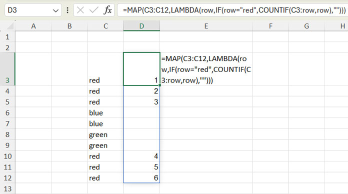
Additional Tip
For the running count of occurrences in Excel, we can also use COUNTIFS. In the above formula, whether it’s a drag-down or dynamic array, feel free to replace COUNTIF with COUNTIFS.
COUNTIFS supports multiple criteria. However, since we only want to specify one criterion (the current row value), we don’t require this function.
That’s why I have opted for COUNTIF, though both functions work.