


How to calculate the number of interest payments aka coupons between the settlement and maturity date of investment, for example, a bond? For this, we can use the COUPNUM function in Google Sheets.
For calculating the number of coupons, other than the settlement and maturity date, we must know the frequency of payments. There are three frequencies. They are;
- Annual.
- Semiannual.
- Quarterly.
One more factor which will affect the calculation is which day count basis to follow.
To calculate the number of interest payments of an investment, you only require the above parameters as input values in the COUPNUM function in Google Sheets.
COUPNUM Function – Syntax and Arguments in Google Sheets
Syntax
COUPNUM(settlement, maturity, frequency, [day_count_convention])Arguments
- settlement – The settlement date of the security, which means the date after issuance (after the issue date) when the security is traded to the buyer.
- maturity – The maturity or expiry of the security.
- frequency – The number of coupon payments per year (refer to table # 1 below).
- day_count_convention – An indicator of what day count basis to follow (refer to table # 2 below). This is an optional argument.
Table # 1 – Frequency
| Frequency Indicator | Coupon (COUPNUM) Basis |
| 1 | Annual |
| 2 | Semiannual |
| 4 | Quarterly |
Table # 2 – Day Count Basis
| Day Count Indicator | Day Count Basis |
| 0 or omitted (default indicator is 0) | US 30/360 as per NASD standards. Which means 30 days in months and 360 days in years. Adjusts the end of month dates according to NASD standards. |
| 1 | Actual/Actual Actual months and actual years. |
| 2 | Actual/360 Actual months but 360 days in years. |
| 3 | Actual/365 Actual months but 365 days in years. |
| 4 | European 30/360 Which means 30 days in months and 360 days in years. Adjusts the end of month dates according to European financial conventions. |
Formula Example to COUPNUM Function in Google Sheets
Here is an example of the use of COUPNUM function in Google Sheets. Forgot to say, this function is available under the ‘Finacial’ category (Insert > Function > Financial) in Google Sheets.
=coupnum(B2,B3,B4,B5)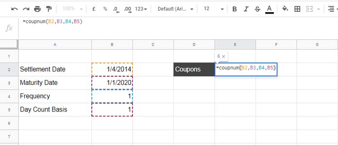
As per the above settlement date, maturity date, and day count basis the semiannual coupon numbers (COUPNUM) will be 12 and quarterly coupon numbers will be 23. You can check that by changing the ‘frequency’ in cell B4 to 2 then 4.
I hope the above example is enough for you to learn the use of COUPNUM function in Google Sheets.
Points to be Noted
How to Properly Input the Settlement and Maturity Dates?
To quickly calculate the coupons, we may use the COUPNUM function in Google Sheets as below.
=coupnum("1/4/2014","1/1/2020",4,1)So we can avoid referring to the cells to feed the arguments. But the above usage, especially the way the settlement date and maturity date is entered, is not recommended.
In all functions, mainly in the financial category functions, use the date inputs using the DATE function.
So when you are not using cell reference in the COUPNUM formula, use it as per the following example.
=coupnum(date(2014,4,1),date(2020,1,1),4,1)Error Values in COUPNUM Function in Google Sheets
- COUPNUM returns the #VALUE! error in the following scenarios.
- Invalid settlement date.
- Invalid maturity date.
For example, the default date format in your sheet is dd/mm/yyyy. If you accidentally insert the settlement or maturity date in mm/dd/yyyy format, you may happen to see the #VALUE! error or wrong coupon numbers.
- COUPNUM returns the #NUM! error in the following cases.
- the frequency is any number other than 1, 2, or 4 (out of range).
- when the day count basis < 0 or > 4 (out of range).
- when settlement ≥ maturity.
That’s all about the use of COUPNUM function in Google Sheets. Enjoy!