


The function AVERAGEIFS does not work inside an ArrayFormula in Google Sheets to return an expanding conditional average of values. The solution is MMULT.
The MMULT approach is not new to my readers. I have already used MMULT to return Average across rows (expanding results without drag and drop). But that doesn’t contain the use of conditions/criteria.
Interested? Here it is – Average Across Rows in Google Sheets.
Here, in this Google Sheets tutorial, I am explaining how to use MMULT as an alternative to AVERAGEIFS ArrayFormula in Google Sheets.
To understand the functions used in writing any of the formulas below, please check my Google Sheets function guide.
Disclaimer:
The formula that I am going to provide on this page may not work in a very large dataset as MMULT has limitations.
My Expectations from an AVERAGEIFS ArrayFormula Output
First I will provide you my sample data and the working non-array AVERAGEIFS formulas. This is to make you understand what output I am expecting.
Then we can go to how to convert that non-array AVERAGEIFS to an array AVERAGEIFS by using MMULT.
Syntax of AVERAGEIFS (for your reference):
AVERAGEIFS(average_range; criteria_range1; criterion1; [criteria_range2; …]; [criterion2; …])Sample Data and Explanation
Here is my Sample Data in which I am going to use to perform the average calculation based on conditions (in a date range).
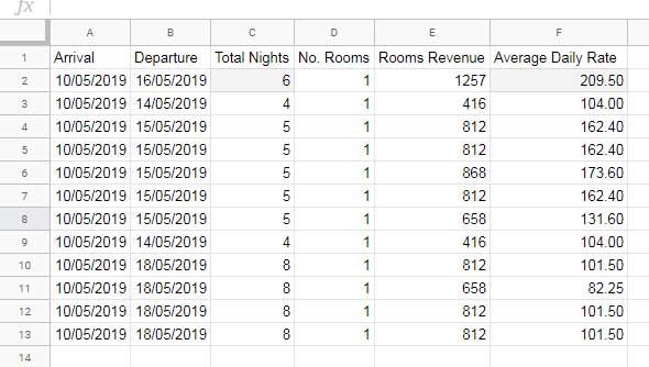
Let’s understand the sample data first that in a limited way.
My sample data above is related to hotel bookings. The columns A and B contain the arrival and departure dates (booked dates) of guests.
Related: Reservation and Booking Status Calendar Template in Google Sheets.
Column C contains the date difference, which means the number of nights booked.
Used the below array formula in cell C2 to populate the date difference aka the number of nights booked.
=ArrayFormula(DAYS(B2:B13,A2:A13))Just understand it (the above DAYS formula) has nothing to do with our AVERAGEIFS array formula in Google Sheets.
The next column is D which is for entering the number of rooms booked.
Column E contains the revenue earned details.
Using the above available details (input) I have calculated the Average Daily Rate (ADR) in column F.
You can search on Google to find more details on ADR. Still here is how to calculate ADR in Google Sheets.
Again all these are part of our sample data. I have not yet started the AVERAGEIFS formula part.
ADR Calculation in Google Sheets
Average Daily Rate (ADR) = Rooms Revenue Earned / No. of Rooms Sold.
As per our sample data columns, ADR is like;
Rooms Revenue (Column E) / No. Rooms (Column D)
Since our revenue includes multiple nights (not a single day) we must use the ADR formula as below.
ADR = Rooms Revenue (Column E) / No. Rooms (Column D) / Total Nights (Column C)
Here is the ADR formula used in cell F3, which is again an array formula.
=ArrayFormula(E2:E13/D2:D13/C2:C13)Our main topic starts below.
Criteria for AVERAGEIFS Calculation and Non-Array Formula
The criteria are in column H and the non-array AVERAGEIFS are in cell I2:I9. The below formula in cell I2 copy-pasted to I3:I9.
=iferror(averageifs($F$2:$F$13,$A$2:$A$13,"<="&H2,$B$2:$B$13,">"&H2))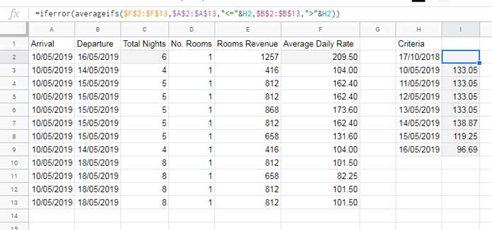
What Does the Averageifs Formula in Cell I2 Do?
If the Arrival dates are less than or equal to the date in H2 and the departure dates are greater than the date in H2, the formula finds the average of the corresponding values from column F (ADR).
That means to find the average of ADR up to the criteria date.
You don’t actually much bother about the criteria or sample data. Just take a look at the AVERAGEIFS formula. That’s enough for us to proceed further.
Let’s see how to replace those formulas (I2:I9) with an AVERAGEIFS ArrayFormula using MMULT in Google Sheets.
Let’s go to the formula now.
MMULT as AVERAGEIFS
Generic AVERAGEIFS Formula:
AVERAGEIFS (ArrayFormula) = SUMIFS (ArrayFormula) / COUNTIFS (ArrayFormula)
First, let’s do the Sumifs part using MMULT.
Remove the non-array AVERAGEIFS formulas from I2:I9. Then insert this MMULT based SUMIFS array formula in cell I2.
=ArrayFormula(iferror(IF(LEN(H2:H),(MMULT(((TRANSPOSE(A2:A)<=H2:H)*(TRANSPOSE(B2:B)>H2:H)),N(F2:F))))))Criteria: The dates from the range H2:H.
The formula checks for ‘Arrival’ date (A2:A) <= criteria date and ‘Departure’ date > criteria date.
We can convert the above SUMIFS to COUNTIFS.
Simply replace the sum column N(F2:F) in the above formula with Row(A2:A)^0 as below.
Insert in cell J2.
=ArrayFormula(iferror(IF(LEN(H2:H),(MMULT(((TRANSPOSE(A2:A)<=H2:H)*(TRANSPOSE(B2:B)>H2:H)),Row(A2:A)^0)))))Based on the generic formula, AVERAGEIFS = SUMIFS / COUNTIFS, here is the AVERAGEIFS ArrayFormula to use in a date range in Google Sheets.
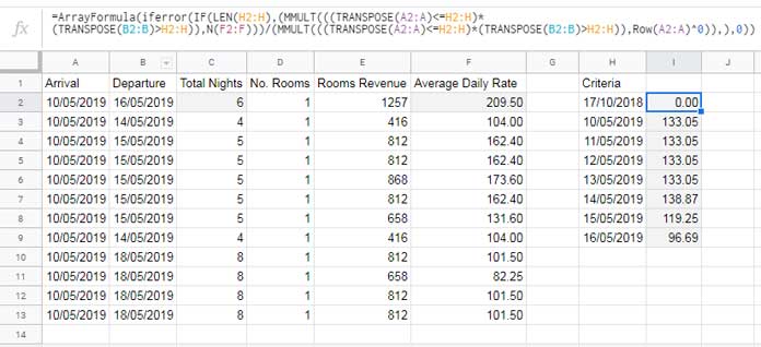
=ArrayFormula(iferror(IF(LEN(H2:H),(MMULT(((TRANSPOSE(A2:A)<=H2:H)*(TRANSPOSE(B2:B)>H2:H)),N(F2:F)))/(MMULT(((TRANSPOSE(A2:A)<=H2:H)*(TRANSPOSE(B2:B)>H2:H)),Row(A2:A)^0)),),0))I have combined the Sumifs and Countifs formulas. Cut the J2 formula and combine (by placing a division operator) with the I2 formula.
The Benefits of the AVERAGEIFS ArrayFormula in Google Sheets
I have already mentioned the limitation of this array formula at the beginning (as a disclaimer) of this post. Now let’s talk about the benefits.
- Just insert the formula in cell I2. It will expand to I2:I9. When you add more criteria in column H it will expand automatically.
- When you insert new rows between the existing range, you must copy-paste a non-array formula. Since our’s is an MMULT based AVERAGEIFS ArrayFormula the question of copy-paste doesn’t exist.
That’s all. Enjoy!