In this tutorial, I’ll explore the differences between the SUMIF function in Excel and Google Sheets.

If you’re familiar with using SUMIF in either platform, you’ll find that approximately 95% of the time, the formulas work seamlessly across both applications. However, some differences can affect how you implement this function.

Basic Use of SUMIF in Excel and Google Sheets

Before diving into the differences, let’s quickly review the basic syntax and usage of SUMIF in both Excel and Google Sheets.

Syntax:

SUMIF(range, criterion, [sum_range])

Here’s a brief explanation of the parameters:

• range: The range of cells that you want to evaluate based on the criterion.
• criterion: The condition that must be met for a cell to be included in the sum.
• sum_range: (Optional) The actual cells to sum if the criterion is met. If this argument is omitted, the function sums the cells in the range.

Similarities in SUMIF Usage

Both Excel and Google Sheets support SUMIF with the same syntax, meaning the fundamental usage of the function is consistent between the two platforms. Many tutorials applicable to Google Sheets will also work in Excel.

Examples of SUMIF in Action

Text Criteria

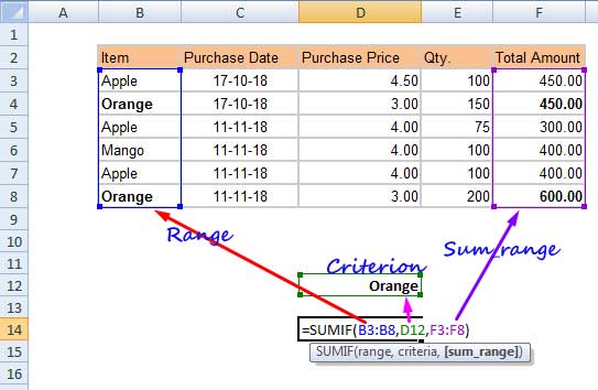
For instance, if you want to sum the values in column F where the item is “Orange,” you would use the following formula:

=SUMIF(B3:B8, "Orange", F3:F8)

This formula sums the values in the cells F4 and F8, where the corresponding cells in column B contain “Orange.”

Alternatively, you can reference the criterion from another cell, such as D12. In that case, the formula would look like this:

=SUMIF(B3:B8, D12, F3:F8)

Date Criteria

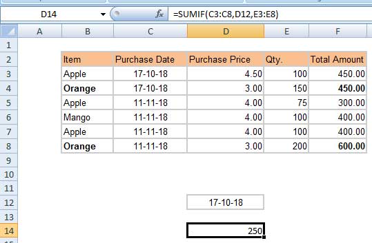
To sum quantities in column E where the purchase date in column C is October 17, 2018, you would set up your formula like this:

=SUMIF(C3:C8, DATE(2018, 10, 17), E3:E8)

If you enter the criterion in cell D12, the formula would be:

=SUMIF(C3:C8, D12, E3:E8)

This approach works the same way in both Excel and Google Sheets, with no notable differences.

Numeric Criteria

For numeric criteria, you can use a cell reference or a hard-coded number:

=SUMIF(E3:E8, 100, F3:F8) // Using hard-coded number
=SUMIF(E3:E8, D12, F3:F8) // Using cell reference

Comparison Operators

The usage of comparison operators (like >, <, =) in SUMIF is also consistent in both applications. For example:

=SUMIF(F3:F7, ">300") // Greater than
=SUMIF(F3:F7, ">=300") // Greater than or equal to
=SUMIF(F3:F7, "<400") // Less than
=SUMIF(F3:F7, "<=400") // Less than or equal to
=SUMIF(F3:F7, 400) // Equal to

Wildcards

Wildcard characters (*, ?, ~) function similarly in both Excel and Google Sheets. They can be used to match patterns in text criteria.

For example, the following SUMIF formula works in both Excel and Google Sheets to sum the values in the range C2:C7 where the corresponding values in B2:B7 end with the word “east”:

=SUMIF(B2:B7, "*east", C2:C7)

Key Differences in SUMIF Functionality

Now, let’s address the differences between the SUMIF function in Excel and Google Sheets:

1. Use of Range

In Excel, the range argument for SUMIF must be a physical range of cells, meaning you cannot use the result of a formula or a dynamic range. In contrast, Google Sheets allows the use of dynamic ranges or formula outputs as the range argument, enhancing its versatility.

Example: Summing by Month

In Google Sheets, you can sum values by month directly using SUMIF with the MONTH function:

=ARRAYFORMULA(SUMIF(MONTH(E3:E7), 5, F3:F7))

In Excel, you would typically use a combination of SUM and IF as follows:

=SUM(IF(MONTH($E$3:$E$7) = 5, $F$3:$F$7, 0)) // Entered as an array formula (Ctrl + Shift + Enter) in older versions of Excel (Legacy array formula)

2. Virtual Ranges

Excel does not support virtual ranges in SUMIF, limiting functionality in some scenarios. For example, cumulative sums using SUMIF with virtual ranges (like using the ROW function) are not possible in Excel but can be done in Google Sheets.

Example: Cumulative Sum in Google Sheets

In Google Sheets, you can easily perform a cumulative sum with:

=ArrayFormula(SUMIF(ROW(A:A), "<=" & ROW(A:A), B:B))

This formula will return the cumulative sum of the values in column B when applied in cell C1.

This approach is not feasible in Excel without using a different method, such as MMULT.

3. Use of Ampersand

Google Sheets allows the use of the ampersand (&) to concatenate strings and criteria within the SUMIF function. For example, if you want to sum quantities based on a combination of values in two columns:

=ArrayFormula(SUMIF(A:A & B:B, "AppleSouth", C:C))

In this example, column A contains fruit names, column B contains regions, and column C contains quantities.

In Excel, this type of concatenation may require additional handling, such as using helper columns or different formulas.

Conclusion

While the SUMIF function in Excel and Google Sheets shares a common foundation, subtle differences in functionality and application can significantly impact your formulas. By understanding these distinctions, you can leverage each platform’s strengths for your data analysis needs.