Ever wondered if there’s a difference between using the INDIRECT function in Excel and Google Sheets?
From my initial experience, the INDIRECT function seemed nearly identical in both platforms. However, as I dug deeper, I discovered some differences worth noting—especially in how each platform handles arrays, named ranges, and certain types of dynamic references.
Here’s a comprehensive comparison of the INDIRECT function in Excel vs. Google Sheets.
Overview of the INDIRECT Function in Excel and Google Sheets
The INDIRECT function returns the cell or range reference specified by a text string, allowing for flexible references within formulas. Both Excel and Google Sheets support the basic use of INDIRECT to reference cells by text. However, there are specific scenarios where they behave differently.
For reference, here’s how the INDIRECT function works in both platforms with basic examples.
Basic Usage: Similarities Between Excel and Google Sheets
In both Excel and Google Sheets, INDIRECT can be used to reference a cell by using a text string as follows:
- Direct Cell Reference
- Suppose cell
A4contains the value 500. - Standard reference:
=A4 - Using INDIRECT:
=INDIRECT("A4")
- Suppose cell
Both formulas will return the value in cell A4 (500) in the target cell.
The INDIRECT function in both platforms opens up new possibilities for creating dynamic references and manipulating data in advanced ways.
Named Ranges with INDIRECT: A Common Feature
Both Excel and Google Sheets support named ranges with INDIRECT. Once a range is named, it can be referenced using INDIRECT by simply entering the name as a text string.
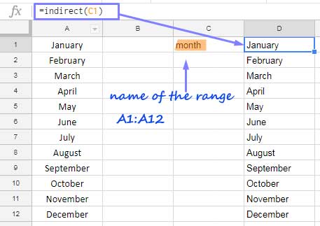
- Example: Name the range
A1:A12as “months.” Then, in any cell, you can use:=INDIRECT("months")
This formula works the same in both Excel and Google Sheets, retrieving the data in the “months” range.
In older versions of Excel, which support legacy array formulas, you might need to enter it as an array formula using Ctrl+Shift+Enter. However, Excel’s dynamic array feature in newer versions has no such requirement.
Differences in Using INDIRECT: Excel vs. Google Sheets
INDIRECT with Array Formulas
One of the notable differences is in how INDIRECT handles array formulas, particularly with named ranges in older versions of Excel:
- Excel (Older Versions): To populate an array using INDIRECT with a named range, Excel requires entering the formula as an array formula, using Ctrl+Shift+Enter (e.g.,
{=INDIRECT("months")}). - Excel (Dynamic Arrays): In newer Excel versions with dynamic arrays, INDIRECT with named ranges automatically expands without needing array formulas.
- Google Sheets: In Google Sheets, INDIRECT expands dynamically by default, so no additional steps are needed to populate a range with a named range.
Example:
Enter “months” (the named range) in cell C1, then use:
=INDIRECT(C1)Google Sheets will return the full range of values in “months” without needing any special array handling.

Cross-Sheet References with INDIRECT
Another difference is the use of INDIRECT for cross-sheet references:
Excel: The following formula works well in Excel to count occurrences of “Apple” across multiple sheets in column A:
=SUMPRODUCT(COUNTIF(INDIRECT(A2:A4&"!$A:$A"), $C$2))Here, A2:A4 contains sheet names (like “Sheet2,” “Sheet3,” etc.), and C2 contains the item to count (“Apple”).

Google Sheets: Google Sheets does not support cross-sheet INDIRECT references in the same way as Excel. To achieve similar functionality, you would need more complex workarounds, such as using the REDUCE Lambda function.
INDIRECT with Dependent Drop-Down Lists
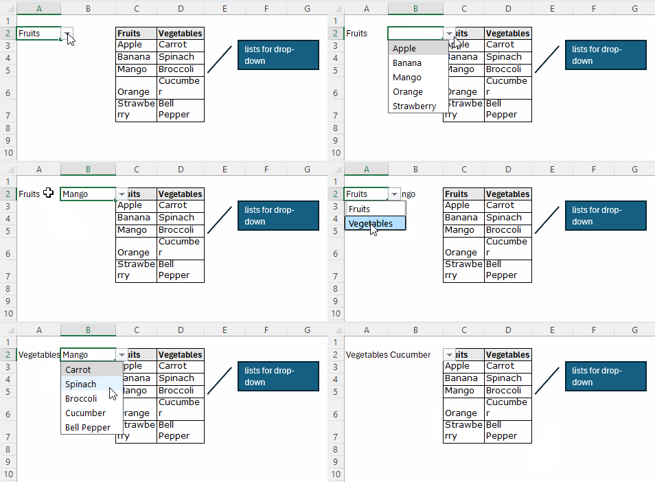
In Excel, INDIRECT is useful for creating dependent drop-down lists:
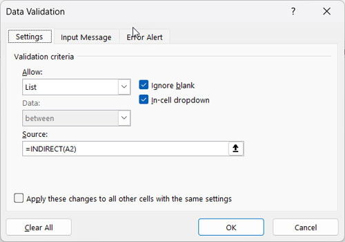
Excel: Suppose you have named ranges “fruits” and “vegetables.” In cell A2, you create a drop-down with “fruits” and “vegetables.” Then, in cell B2, using =INDIRECT(A2) in the data validation list will create a dependent drop-down that shows either the list of fruits or vegetables based on the selection in A2.

You can copy and paste these drop-downs to the rows below to create multi-row dynamic dependent drop-downs.
Google Sheets: Google Sheets requires a workaround to create multi-row dynamic dependent drop-downs. Custom scripts or the Data Validation feature combined with complex formulas are often necessary.
Note: This difference is related to data validation functionality rather than an issue with the INDIRECT function itself. Excel supports INDIRECT directly in data validation for dependent lists, while Google Sheets does not.

Summary of INDIRECT Differences in Excel vs. Google Sheets
| Feature | Excel | Google Sheets |
| Basic Cell Reference | Supported | Supported |
| Named Ranges | Supported | Supported |
| Array Formulas (Older Excel) | Requires Array Formula | Expands by default |
| Dynamic Arrays (New Excel) | Expands by default | Expands by default |
| Cross-Sheet References | Fully Supported | Limited, requires workarounds |
| Dependent Drop-Down Lists | Easy with INDIRECT | Requires script/workaround |
Conclusion
While both Excel and Google Sheets support the basic functionality of INDIRECT, they differ in how they handle advanced applications like cross-sheet references, array formulas, and dependent drop-down lists. These differences are primarily due to Excel’s legacy array formula requirements and Google Sheets’ limited support for cross-sheet dynamic references.
For users primarily working in Excel, INDIRECT is a powerful tool for dynamic data manipulation across sheets and dependent lists. Google Sheets users can achieve similar results but may need to rely on more complex formulas or Google Apps Script for advanced uses.
If you discover any other differences in using INDIRECT in Excel vs. Google Sheets, feel free to share!


Here’s an example where this function differs slightly based on which application you are using.
Works in Google Sheets written as:
=COUNTA(INDIRECT("'"&A1&"'!A2:A"))Will need to be re-written in excel as:
=COUNTA(INDIRECT("'"&A1&"'!A:A"))-1Hi, Chris,
Thanks for the tip.