To unpivot a calendar grid in Google Sheets (i.e., repeat each date for every entry under it), use the following dynamic formula:

=ARRAYFORMULA(LET(
  calendar, B4:H33,
  nRowsInWeek, 5,
  nColsPerDay, 1,
  nDtRows, 6,
  DtColId, XMATCH(SEQUENCE(nDtRows*nRowsInWeek), SEQUENCE(nDtRows,1,1,nRowsInWeek)),
  dts, CHOOSECOLS(FILTER(calendar, DtColId), SEQUENCE(1,7,1,nColsPerDay)),
  srDts, SEQUENCE(nDtRows),
  srDtsRpt, INT(SEQUENCE(nDtRows*(nRowsInWeek-1),1,1,1/(nRowsInWeek-1))),
  allDts, TOCOL(VLOOKUP(srDtsRpt, HSTACK(srDts,dts), SEQUENCE(1,7,2), FALSE)),
  allData, WRAPROWS(TOCOL(FILTER(calendar, NOT(IFNA(DtColId)))), nColsPerDay),
  ftr, FILTER(HSTACK(allDts, allData), allDts>0),
  SORT(ftr, 1, 1, SEQUENCE(ROWS(ftr)), 1)
))

This Google Sheets unpivot formula converts a calendar grid into a clean, row-wise table by repeating each date for every corresponding entry. The resulting structure makes your data much easier to filter, sort, and analyze.

Introduction to Unpivoting a Calendar Grid in Google Sheets

Calendar-style data in Google Sheets is easy to read and widely used. However, it becomes difficult to analyze because the data is spread across multiple columns and visually grouped by dates.

In a typical calendar grid in Google Sheets:

• Dates appear across columns
• Each date may contain multiple rows (and sometimes multiple columns) of data beneath it

While this layout works well for viewing schedules, tasks, or logs, it is not suitable for data analysis.

This is where you need to unpivot the calendar grid.

In this tutorial, you’ll learn how to unpivot a calendar grid in Google Sheets by repeating each date for every entry under it. This converts the layout into a clean, row-wise table that is ideal for filtering, sorting, and reporting.

Why This Unpivot Method Works in Google Sheets

The best part? This Google Sheets unpivot method is fully dynamic and works even when:

• Each week contains multiple rows of data (the number of rows must be consistent across all weeks). For example, 5 data rows under each date row.
• Each date spans multiple columns (such as merged cells across two or more columns), as long as it is consistent across all dates
• The calendar follows a standard 7-day grid

Example 1: Unpivot a Standard Calendar Grid (One Column per Day)

Let’s start with a standard calendar grid in Google Sheets, where each day occupies a single column.

Key Points About This Layout

• The calendar contains 6 date rows (rows 4, 7, 10, 13, 16, and 19).
• Each week consists of 3 rows:
  • 1 row for dates
  • 2 rows for data
• You can use more data rows per week, but the number of rows must remain consistent across all weeks.
• The data range is B4:H21 (excluding the weekday headers).

Update the Formula Parameters

To unpivot this calendar grid in Google Sheets, update the following parameters in the formula:

Original:

calendar, B4:H33,
nRowsInWeek, 5,
nColsPerDay, 1,
nDtRows, 6,

Updated:

• calendar → B4:H21
• nRowsInWeek → 3 (1 date row + 2 data rows)
• nColsPerDay → 1 (one column per day)
• nDtRows → 6 (total number of date rows)

Final Formula

=ARRAYFORMULA(LET(
  calendar, B4:H21,
  nRowsInWeek, 3,
  nColsPerDay, 1,
  nDtRows, 6,
  DtColId, XMATCH(SEQUENCE(nDtRows*nRowsInWeek), SEQUENCE(nDtRows,1,1,nRowsInWeek)),
  dts, CHOOSECOLS(FILTER(calendar, DtColId), SEQUENCE(1,7,1,nColsPerDay)),
  srDts, SEQUENCE(nDtRows),
  srDtsRpt, INT(SEQUENCE(nDtRows*(nRowsInWeek-1),1,1,1/(nRowsInWeek-1))),
  allDts, TOCOL(VLOOKUP(srDtsRpt, HSTACK(srDts,dts), SEQUENCE(1,7,2), FALSE)),
  allData, WRAPROWS(TOCOL(FILTER(calendar, NOT(IFNA(DtColId)))), nColsPerDay),
  ftr, FILTER(HSTACK(allDts, allData), allDts>0),
  SORT(ftr, 1, 1, SEQUENCE(ROWS(ftr)), 1)
))

Result

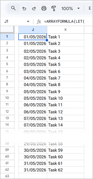
• The output contains 2 columns → Date | Task
• Each date is repeated for every corresponding entry, effectively converting the calendar into a row-wise table

Note: Structured sample data is used here to clearly demonstrate how to unpivot a calendar in Google Sheets and understand the transformation.

Example 1.1: Unpivot Calendar with Different Rows per Week and Date Rows

In the previous example, we worked with a May 2026 calendar, which contains 6 date rows.

In this example, we’ll use a February 2025 calendar, which has only 5 date rows. Additionally, each week contains 2 rows:

• 1 row for dates
• 1 row for data

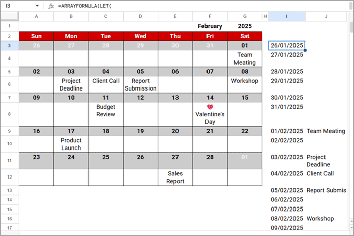
The calendar range is A3:G12 (excluding the header row).

Update the Parameters

To correctly unpivot this calendar grid in Google Sheets, update the formula parameters as follows:

calendar, A3:G12,
nRowsInWeek, 2,
nColsPerDay, 1,
nDtRows, 5,

Why These Changes Matter

• nRowsInWeek → 2 ensures the formula correctly identifies one date row and one data row per week
• nDtRows → 5 matches the total number of date rows in the calendar
• calendar → A3:G12 defines the correct data range for this layout

By adjusting these parameters, the same Google Sheets unpivot formula dynamically adapts to different calendar structures while still repeating each date for every entry.

Example 2: Unpivot a Calendar Grid with Multiple Columns per Day

In some cases, each date in a calendar grid in Google Sheets may span multiple columns instead of just one.

For example:

• Column 1 → Task
• Column 2 → Status

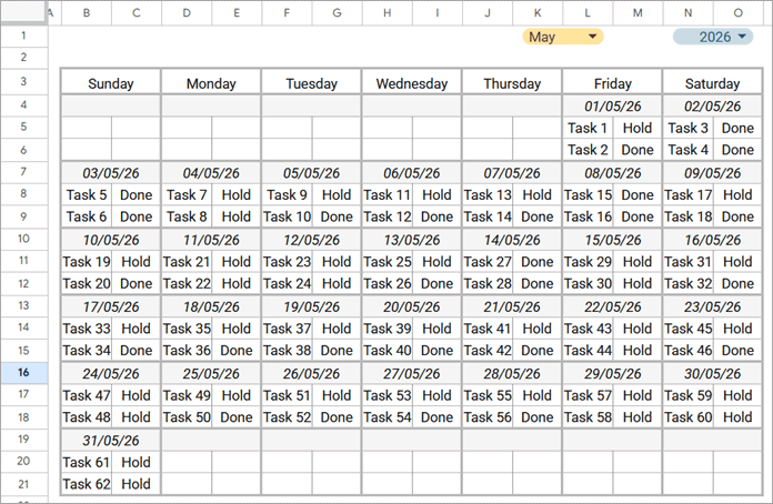
What Changes When Each Date Has Multiple Columns?

Since each date now contains multiple columns, the unpivoted output will expand accordingly:

• Column 1 → Date
• Column 2 → Task
• Column 3 → Status

This allows you to flatten the calendar data in Google Sheets while preserving all related fields for each entry.

Update the Parameters

To unpivot a calendar with multiple columns per day, update the formula parameters as follows:

calendar, B4:O21,
nRowsInWeek, 3,
nColsPerDay, 2,
nDtRows, 6

• nColsPerDay → 2 ensures both columns (e.g., Task and Status) are included for each date
• calendar → B4:O21 expands the range to cover all columns

Final Formula

=ARRAYFORMULA(LET(
  calendar, B4:O21,
  nRowsInWeek, 3,
  nColsPerDay, 2,
  nDtRows, 6,
  DtColId, XMATCH(SEQUENCE(nDtRows*nRowsInWeek), SEQUENCE(nDtRows,1,1,nRowsInWeek)),
  dts, CHOOSECOLS(FILTER(calendar, DtColId), SEQUENCE(1,7,1,nColsPerDay)),
  srDts, SEQUENCE(nDtRows),
  srDtsRpt, INT(SEQUENCE(nDtRows*(nRowsInWeek-1),1,1,1/(nRowsInWeek-1))),
  allDts, TOCOL(VLOOKUP(srDtsRpt, HSTACK(srDts,dts), SEQUENCE(1,7,2), FALSE)),
  allData, WRAPROWS(TOCOL(FILTER(calendar, NOT(IFNA(DtColId)))), nColsPerDay),
  ftr, FILTER(HSTACK(allDts, allData), allDts>0),
  SORT(ftr, 1, 1, SEQUENCE(ROWS(ftr)), 1)
))

Result

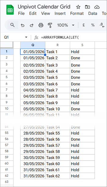
• The output now includes multiple columns per entry, such as Date, Task, and Status
• Each date is repeated for every corresponding row of data, while keeping all columns properly aligned

This approach ensures you can unpivot a calendar grid in Google Sheets by repeating dates for each entry, even when each date contains multiple fields.

How the Formula Unpivots (Flattens) a Calendar Grid in Google Sheets

This Google Sheets unpivot formula dynamically flattens a calendar grid into a row-wise structure using the following logic:

Step-by-Step Breakdown of the Unpivot Formula

DtColId
Generates sequential numbers for the date rows and returns #N/A for the data rows below them.
This acts as an identifier to separate date rows from data rows in the calendar.

dts
Filters only the date rows from the calendar.

Additionally, when each date spans multiple columns (as in Example 2), it selects only the required columns to reconstruct a proper 7-column calendar grid.

srDts
Creates a sequence based on the total number of date rows in the calendar.

srDtsRpt
Repeats the sequence generated by srDts based on the number of data rows per week (nRowsInWeek - 1).

For example, if:

• Date rows = 1 to 6
• Rows per week = 3

The result will be:

1
1
2
2
3
3
4
4
5
5
6
6

Each date row index is repeated based on the number of data rows.

allDts
Uses the repeated sequence (srDtsRpt) to look up and repeat the actual dates from the calendar, then flattens them into a single column.

This step ensures that each date is duplicated for every corresponding data row, creating a column of repeated dates required to unpivot the calendar data in Google Sheets.

allData
Filters the data rows and reshapes them into a row-wise structure. When multiple columns exist per date, it preserves those columns for each entry.

ftr
Combines the repeated dates (allDts) with the corresponding data (allData) and removes any empty rows.

Final Step (SORT)
Sorts the output to ensure that dates and their corresponding entries are properly aligned and ordered after the calendar is flattened in Google Sheets.

This structured approach allows you to convert a calendar grid into a normalized table, making it much easier to analyze, filter, and report on your data.

FAQs

Can I use this formula for any month and year?

Yes, you can use this Google Sheets calendar unpivot formula for any month and year.

If a month contains fewer weeks (fewer date rows), simply adjust the nDtRows parameter in the formula accordingly.

Can I use a different number of rows per week?

Yes, you can. However, the number of rows per week must remain consistent across all weeks in the calendar grid for the formula to work correctly.

Can this handle merged cells?

Yes. This method works even if your calendar uses merged cells, as long as you correctly define:

• nColsPerDay (number of columns per date)

This ensures the formula correctly captures all columns associated with each date.

Why do I see dates from the previous or next month?

In a standard calendar grid in Google Sheets, you may see dates from the previous or next month.

This happens because calendar layouts often include preceding and succeeding month dates to maintain a complete 7-day week structure.

For example:

• The first week of a month may include dates from the previous month
• The last week may include dates from the next month

When you unpivot the calendar, these dates are also included and repeated along with their corresponding entries.

If needed, you can filter the results to include only the target month after unpivoting. For example, you can use a FILTER function to include only dates from the current month.

Can I use this with real-world data?

Absolutely. You can use this approach to flatten calendar data in Google Sheets for various real-world scenarios, such as:

• Task tracking
• Shift schedules
• Attendance logs
• Sales or inventory data

Conclusion: Unpivoting a Calendar Grid in Google Sheets

Unpivoting a calendar grid in Google Sheets allows you to convert visually structured data into an analysis-friendly, row-wise format.

With this dynamic formula, you can:

• Repeat dates for each entry
• Handle multiple rows and columns per date
• Work with standard calendar layouts

This makes it much easier to filter, sort, and analyze data, or even create pivot tables and dashboards.

If you regularly work with calendar-based data, learning how to unpivot a calendar in Google Sheets can significantly improve your data analysis workflow.

Related Google Sheets Tutorials

• Filter a Custom Calendar with Events in Google Sheets – View filtered events in calendar format or as a structured table for analysis
• Filter Today’s Events from a Calendar Layout in Google Sheets – Quickly extract events for the current day
• Convert Google Sheets Calendar into a Table – Converts calendar data into a structured table without repeating dates