


")


")

")
")
 in Excel & Google Sheets")


You may often need to sum text values in Google Sheets by virtually assigning numerical scores to them. This is especially common in surveys, feedback forms, or performance assessments.
For example, you may have a table of product feedback from users, where ratings are given as text responses like:
“Exceptional”, “Very Good”, “Good”, “Fair”, and “Very Poor”
Each of these text values can be mapped to scores such as 5, 4, 3, 2, and 1 respectively.
But how do you calculate total or average scores from these text-based responses?
Let’s explore how to sum text values by mapping scores in Google Sheets using two real-world examples.
Example 1: Calculate Scores from Text Responses (User Ratings)
Here’s a simple table of product feedback collected from users:
| User | Response |
|---|---|
| Maria | Excellent |
| James | Good |
| Charlie | Fair |
| Olivia | Poor |
| Evan | Excellent |
| Amelia | Good |
| Oliver | Poor |
Assume we map the rating text to the following scores:
| Text Response | Score |
|---|---|
| Excellent | 5 |
| Good | 4 |
| Fair | 3 |
| Poor | 2 |
To calculate scores from the text responses, use the formula below. Assuming your table is in range A1:B, with headers in row 1, enter this formula in cell C2:
=SWITCH(B2:B, "Excellent", 5, "Good", 4, "Fair", 3, "Poor", 2, IFERROR(1/0))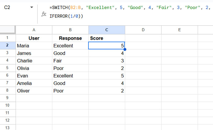
This formula maps each text to its corresponding score. The IFERROR(1/0) trick returns a blank (error) instead of 0 for any unmatched or empty responses, ensuring cleaner averages.
To calculate the average score from these text values:
=AVERAGE(
   SWITCH(B2:B, "Excellent", 5, "Good", 4, "Fair", 3, "Poor", 2, IFERROR(1/0))
)
To sum the text values instead:
=SUM(
   SWITCH(B2:B, "Excellent", 5, "Good", 4, "Fair", 3, "Poor", 2, IFERROR(1/0))
)
This is how you can sum text values by mapping scores in Google Sheets for feedback-type data.
Example 2: Sum Text Values (Student Performance) by Mapping Scores in Google Sheets
Suppose you have a table with students’ test ratings given as text values:
| Name | Test 1 | Test 2 | Test 3 | Total Score |
|---|---|---|---|---|
| Christina | Exceptional | Good | Exceptional | |
| James | Very Good | Very Good | Exceptional | |
| Bobby | Very Poor | Very Poor | Fair | |
| Amy | Fair | Fair | Fair |
Let’s say we want to sum each student’s score based on this mapping:
| Text Response | Score |
|---|---|
| Exceptional | 5 |
| Very Good | 4 |
| Good | 3 |
| Fair | 2 |
| Very Poor | 1 |
Since text can’t be summed directly, we’ll map each value to its corresponding score using SWITCH.
Method 1: Row-by-row sum using SWITCH
In cell E2, enter:
=SUM(
   SWITCH(B2:D2, "Exceptional", 5, "Very Good", 4, "Good", 3, "Fair", 2, "Very Poor", 1, IFERROR(1/0))
)
Drag this down to fill the entire column. This will sum scores for each student based on their test responses.
Method 2: Use BYROW and LAMBDA (no dragging)
To apply the logic across the entire range automatically:
=BYROW(B2:D, LAMBDA(row,
   SUM(
      SWITCH(row, "Exceptional", 5, "Very Good", 4, "Good", 3, "Fair", 2, "Very Poor", 1, IFERROR(1/0)))
   )
)
This outputs a column of total scores row-wise. But it might return trailing 0s for empty rows.
To return blank instead of 0s:
=BYROW(B2:D, LAMBDA(row,
   LET(score,
      SUM(
         SWITCH(row, "Exceptional", 5, "Very Good", 4, "Good", 3, "Fair", 2, "Very Poor", 1, IFERROR(1/0))), IF(score=0,,score)
      )
   )
)
Conclusion
When working with survey responses, feedback, or performance ratings stored as text, you can easily sum text values by mapping scores in Google Sheets using SWITCH, SUM, BYROW, and LAMBDA.
This approach helps you extract meaningful numerical summaries from qualitative input without manual conversion.
Amazing Prashnath!! Thank you so much for this.
Is there a way that the formula brings the most common word/text used??
I’m doing a matrix to prioritize features. I’m using a “must-have won’t have” criteria.
In the end, if we have more “must-haves,” we will do it.
Rather than having the output, this is a 95 score feature.
Does that make sense?? thanks in advance
Hi, Luiz Gattaz,
I don’t know how your data is formatted. I assume the said two strings are spread in the range B2:D10.
If so, insert the below formulas in F2 and G2, respectively.
F2
=UNIQUE(flatten(B2:D10))G2
=ArrayFormula(countif(flatten(B2:D10),unique(flatten(B2:D10))))If that doesn’t help, feel free to share a sample sheet via “Reply” below. I won’t make it public.
Thanks for this! I’m using this in our employees’ leave tracker. However, whenever I add the SUM function, I get an error ‘did not find value in VLOOKUP evaluation’ I’m not sure what’s wrong.
Hi, Jenny,
To verify your formula personally, you can consider leaving your sheet link via “Reply”. Before publishing, I will remove the link from your reply.
Thanks for this, has been very helpful. I’m using it to automatically score a multiple-choice test from google forms where each multiple-choice has a different score (not just right or wrong).
The trouble I’m having now is that the cell with the formula seems to be deleted each time a new form is submitted, therefore it doesn’t auto-complete. Do you know why this could be?
Hi, Ed,
Avoid using any formula in the ‘form response’ tab. It may cause issues with array formulas.
As a solution, add a new sheet tab and do your data manipulation on that.
For example, if your form response tab and data range is
'form response'!A1:D, in the newly added sheet use the below formula in cell A1.={'form response'!A1:D}