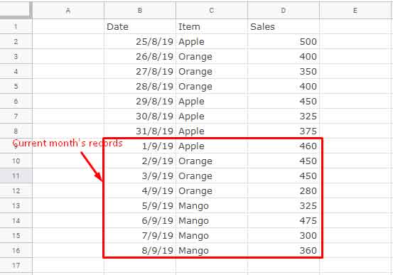
We can use the MONTH(), YEAR(), and NOW() functions to sum current month data using the QUERY function in Google Sheets. Compared to using specific date criteria, applying these scalar functions in QUERY is actually easier.

Summing by the current month using QUERY is quite straightforward.

Let’s walk through it step by step. First, we’ll filter by the current month using QUERY. Then, we’ll sum the current month’s values in Google Sheets.

This tutorial is part of the Date Logic in QUERY hub.
Learn how date logic works in Google Sheets QUERY, including date criteria, month-based filtering, and DateTime handling.

Sample Data

Just a note: when I wrote this post, the current month was September and the year was 2019.

Google Sheets: Sum Current Month Data Using QUERY Function

The Role of YEAR(), MONTH(), and NOW() Scalar Functions to Filter Current Month Records

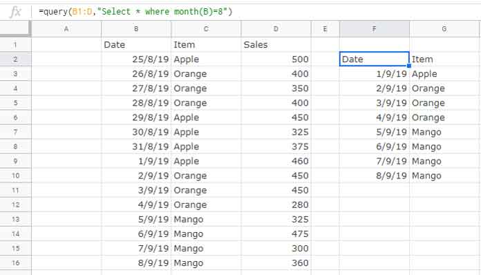
To filter data for a specific month, you can use the MONTH() function like this:

=QUERY(B1:D, "SELECT * WHERE MONTH(B) = 8")

This formula filters records that fall in September.

Why 8 for September? In the QUERY language in Google Sheets, months are zero-indexed — meaning January is 0, February is 1, and so on. So, 8 represents September, not August.

To filter dynamically for the current month, replace 8 with MONTH(NOW()):

=QUERY(B1:D, "SELECT * WHERE MONTH(B) = MONTH(NOW())")

But here’s a catch: the formula only checks the month, not the year. So if a date like 08/09/2020 (8th September 2020) is present, and the current year is 2019, that record would still be included — even though it’s from a different year.

To fix this, we need to check both the MONTH() and YEAR() in the QUERY formula.

=QUERY(B1:D, "SELECT * WHERE MONTH(B) = MONTH(NOW()) AND YEAR(B) = YEAR(NOW())")

This formula ensures that only the records from the current month and year are included.

QUERY to Sum Current Month Records in Google Sheets

Now that you know how to filter the current month’s data, summing it is easy. Just replace the asterisk (*) in the SELECT clause with SUM(D) (assuming column D contains the values to sum):

=QUERY(B1:D, "SELECT SUM(D) WHERE MONTH(B) = MONTH(NOW()) AND YEAR(B) = YEAR(NOW())")

Conditionally Sum Current Month Data Using QUERY in Google Sheets

It’s also simple to add conditions to your QUERY formula.

Let’s say you want to sum the current month’s sales of the item “Orange.” Here’s the formula:

=QUERY(B1:D, "SELECT SUM(D) WHERE C = 'Orange' AND MONTH(B) = MONTH(NOW()) AND YEAR(B) = YEAR(NOW())")

Want to add one more condition to the current month sum?

Here’s how you can sum values based on multiple conditions:

Formula to Sum Current Month’s Records Based on Two or More Criteria

For example, if you want to sum sales where the item is either “Orange” or “Mango,” and the date falls in the current month and year:

=QUERY(B1:D, "SELECT SUM(D) WHERE (C = 'Orange' OR C = 'Mango') AND (MONTH(B) = MONTH(NOW()) AND YEAR(B) = YEAR(NOW()))")

That’s all! Do you have any questions about how to sum current month data using QUERY in Google Sheets? Feel free to drop them in the comments. Enjoy!

Resources

• Finding the First and Last Workdays of a Month in Google Sheets