Are you looking for a way—perhaps using a regular expression—to remove repeated characters from the end of strings in Google Sheets? You’re in the right place!
Let me first explain the context. When combining multiple values in Google Sheets, we often use delimiters like ~ (tilde), | (pipe), / (forward slash), or ^ (caret) to separate values. These characters are called delimiters.
However, when the source cells contain blank values, these delimiters can appear unnecessarily at the end of the resulting string. That’s where things get messy.
Let’s take an example.
Unwanted Characters at the End of a String in Google Sheets
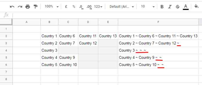
Say we’re combining the values from columns B to E (range B2:E6), and placing the result in column F, starting from cell F2. The result might look something like this:

You can see the unwanted, repeated tilde characters (~) at the end. I want to remove these only from the end of the string, without affecting any delimiter in the middle.
Depending on how you join the values, there may or may not be spaces around the delimiter. In this example, we’ve used " ~ " with a single space on either side. So even though the delimiters look consecutive, they are technically not, because of the spacing.
To complicate things further, we don’t know how many delimiters will appear at the end—it depends entirely on how many source cells are blank.
So, how do we clean this up and remove repeated characters from the end of strings in Google Sheets?
Before and After
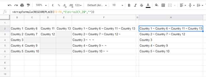
Here’s a visual of what we’re trying to do:
Before
Country 4 ~ Country 9 ~ ~
After
Country 4 ~ Country 9
Step 1: Combine Columns with Delimiters
This tutorial focuses on cleaning up delimiters, but first, here are a few ways to combine columns.
- Formula 1 – Basic formula for one row (in
F2):
=B2&" ~ "&C2&" ~ "&D2&" ~ "&E2- Formula 2 – ArrayFormula version for multiple rows (in
F2):
=ArrayFormula(B2:B6&" ~ "&C2:C6&" ~ "&D2:D6&" ~ "&E2:E6)- Formula 3 – Dynamic array formula (in
F2):
=ArrayFormula(TRANSPOSE(QUERY(TRANSPOSE(B2:E6&" ~ "),,9^9)))This third option is cleaner and more scalable, but it comes with a caveat that we’ll cover in the conclusion — so hold off on using it for now.
Step 2: Remove Repeated Characters from the End of Strings in Google Sheets
Now let’s remove those repeated delimiters.
The best tool for this task is REGEXREPLACE. Why?
REPLACErequires you to know the position and length (not helpful here).SUBSTITUTEdoesn’t let you target the end of a string.REGEXREPLACEworks great for flexible pattern matching.
Formula to Remove Consecutive Delimiters at the End
For individual cells (in G2):
=REGEXREPLACE(F2, "(\s\~\s){1,}$","")ArrayFormula for multiple cells (in G2):
=ArrayFormula(REGEXREPLACE(F2:F6, "(\s\~\s){1,}$",""))
This removes one or more occurrences of " ~ " only from the end of the string.
If you don’t use spaces around the delimiter, and your string looks like this:Country 1~Country 6~Country 11~Country 13~~,
then use the pattern:
=REGEXREPLACE(F2, "(\~){1,}$", "")Explanation of the Regex Pattern
The pattern we used: (\s\~\s){1,}$
\s– Matches a whitespace character.\~– Matches the tilde~.{1,}– Quantifier that matches one or more occurrences.$– Anchors the match to the end of the string.
If you’re using other delimiters, here are the corresponding patterns:
- For
^:(\s\^\s){1,}$ - For
/:(\s\/\s){1,}$ - For
|:(\s\|\s){1,}$
Replace ~ with the delimiter you use.
A Note on Formula 3
We didn’t apply the REGEXREPLACE to Formula 3 earlier. Why?
That formula tends to add inconsistent spaces around the delimiter, making it harder to match with a regex. But with a small tweak, you can still clean it up:
Update the formula to avoid irregular spacing as follows:
=ArrayFormula(TRANSPOSE(QUERY(TRANSPOSE(B2:E6 & " ~"), , 9^9)) & " ")That’s It!
You’ve now learned how to remove repeated characters from the end of strings in Google Sheets using REGEXREPLACE. This technique keeps your results clean and professional, especially when combining data with delimiters.


