


")


")

")
")
 in Excel & Google Sheets")


Google Sheets now lets you unlock rows and columns when using “Drop-down (from a range)”—a big improvement if you’ve ever tried to create dependent drop-downs without scripts. This new feature basically lets us use relative reference in drop-down in Google Sheets, instead of being stuck with fixed (absolute) references.
Earlier, any drop-down created from a range would always refer to the same range—no matter where you copied it. But now, we can control whether that range shifts when the drop-down is copied or dragged to other cells.
Let’s break it down with examples.
Why Relative Reference Matters in Drop-Downs
Let’s say you have a drop-down in cell E10. When you click it, you see a list of values from another range.
Before this update, if you copied that drop-down to E11, it would still refer to the original range—like E1:E4—not a new one. That’s because Google Sheets was treating the range as an absolute reference by default.
But now, with the new relative reference in drop-down in Google Sheets, you can let the range shift dynamically when the drop-down is copied or dragged. This is especially helpful when building multi-row dependent drop-downs.
A quick note on terminology:
- Drop-down = manually entered list of values
- Drop-down (from a range) = list pulled from a range of cells
Let’s see both absolute and relative references in action.
Example 1: Absolute Reference (Locked Range)
This is the default behavior in Google Sheets.
1. In cells E1:E4, enter:
Approved
Pending
Rejected
Incomplete
2. Select B5, then go to Insert > Drop-down or Data > Data validation > +Add rule
3. Under Criteria, choose Drop-down (from a range) and enter E1:E4
4. Click Done
Now you’ll see that B5 has a drop-down with those four values. If you copy B5 to B6, both will pull from the same range—E1:E4—because the reference is locked.
Example 2: Relative Reference (Unlocked Range)
Now let’s create a drop-down where the range changes automatically as we move the drop-down to a different row.
1. In range E2:G5, enter these month values:
| Jan | Feb | Mar |
| Apr | May | Jun |
| Jul | Aug | Sept |
| Oct | Nov | Dec |
2. Select B2, then go to Insert > Drop-down or Data > Data validation > +Add rule
3. Under Criteria, choose Drop-down (from a range)
4. In the range field, enter: =E2:G2 (Make sure to include the = sign. If you don’t, Sheets may treat it as an absolute reference.)
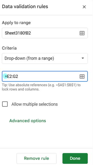
5. Click Done, then copy B2 down to B3, B4, and B5
Now each drop-down is linked to a different row:
- B2 → E2:G2
- B3 → E3:G3
- B4 → E4:G4
- B5 → E5:G5
That’s exactly how relative reference in drop-down in Google Sheets is supposed to work.
Note: If your range is on a different sheet, include the sheet name like this:=Sheet2!E2:G2
This ensures the drop-down can correctly reference the values across sheets.
Summary: Relative vs. Absolute Drop-Downs
Here’s a quick comparison of how the two behave:
| Type of Reference | Behavior |
|---|---|
| Absolute | The range doesn’t change when copied (e.g., always E1:E4) |
| Relative | The range updates based on where the drop-down is pasted (e.g., E2:G2 → E3:G3) |
To enable relative reference, just use an equal sign like =E2:G2 when setting the range.