Padding Values with Spaces to Make Them Equal in Length in Sheets

Normally most of your strings in cells will be of different length unless the cells contain identical values. To make them equal length, you can add trailing spaces. Before padding values with spaces in Google Sheets, you must understand one thing. What’s that?

You may need to add a different number of spaces to each value. Because the length of the values may differ in each row.

I will explain to you how to address such issues with a Len array formula and Max. Also, my formula is multi-column compatible. Before that let me show you how padding values with spaces are useful (in rare cases though).

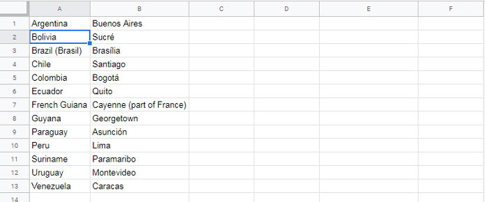
The Values to Pad:

Sample data for padding values with spaces in Google Sheets

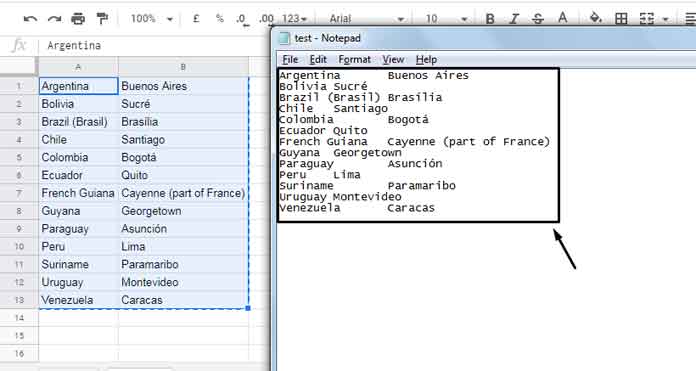
I am copying this two column data to Notepad. See how the pasted values look! It’s almost difficult to understand/read.

Notepad output before padding equal space

With padding values with the space characters, you can sort out the above problem. You pad values in column A and B with spaces to make them equal in length. Then when you copy and paste, it would correctly be arranged, I mean like a tabular form.

Notepad output after padding equal space

Steps Involved in Padding Values with Spaces in Google Sheets

Let me teach you how to code the formula for this in 4 simple steps.

We can use the function LEN to find the length of a string in a cell. For example, to find the length of the string in cell A1 we can use the below formula.

=len(A1)

It would return 9 as the value in cell A1 is “Argentina” which is 9 characters long. This is not what we want. First what we want is to find the maximum length of the values in the range A1:A.

Step 1:

Array Formula to Find the Length of All the Strings in a Column

You can use the LEN function in an array as below.

=ArrayFormula(len(A1:A))

It will return the length of all the values in the range in row-wise. Just enter this formula in any blank column and see the output. Then you can remove this formula. We can use this later with another formula.

Step 2:

Find the Maximum Length of the Strings in a Column

Use the Max function together with the above Len Array Formula to return the maximum length of the strings in column A.

This time also just enter this formula in any cell and see the output. Then delete it.

=ArrayFormula(max(len(A1:A)))

Step 3:

Find the Number of Spaces to Add to the Values in Each Row

We have found the maximum length of values in column A (Step 2) and also the length of each string in rows (Step 1) in that column.

So now we can easily find the number of spaces to add to each string. How?

It’s like;

(Formula in Step 2 - Formula in Step 1)

It other words;

=ArrayFormula(max(len(A1:A)))-ArrayFormula(len(A1:A))

Wait! It won’t work unless you restructure the array formula correctly. No need to use multiple Array Formulas in a combo. Here is the correct formula.

=ArrayFormula(max(len(A1:A))-len(A1:A))

Step 4:

Formula for Padding Values with Spaces in Google Sheets

In the just above step we coded a formula to find the number of spaces to add to values in each row in column A. Now let me show you how to add spaces, I mean padding values with spaces.

You can repeat the space character as many numbers of times as you want using the Rept function in Sheets.

The just above formula returns the number of times to repeat the space character. So we can use that in the Rept formula as below.

=ArrayFormula(rept(" ",max(len(A1:A))-len(A1:A)))

The above formula populates spaces in each row based on the length of the values in column A. So just combine this formula with the values in A2:A to add spaces to each value.

=ArrayFormula(A1:A&rept(" ",max(len(A1:A))-len(A1:A)))

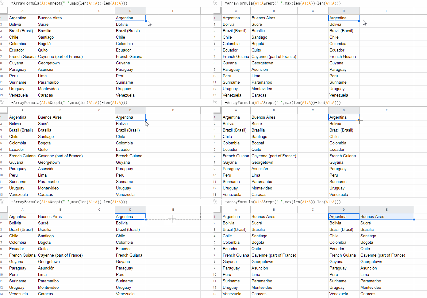
This time you can keep this formula in cell D1. Then drag this formula to the right. It will add an equal number of spaces to the values in column B too!

Padding values with spaces in Google Sheets - Array Formula

If you have values in column C also, you can drag the formula to the right even further. I mean you can drag the formula from D1 to F1.

Copy the values in column E1:D to Notepad. You can see that it’s correctly padded.

That’s all for now.

Prashanth KV
Prashanth KV
Your Trusted Google Sheets and Excel Guide Prashanth KV brings a wealth of experience in Google Sheets and Excel, cultivated through years of work with multinational corporations in Mumbai and Dubai. As a recognized Google Product Expert in Docs Editors, Prashanth shares his expertise through insightful blogging since 2012. Explore his blog for practical tips and guidance on maximizing your spreadsheet skills.

Compare Two Tables for Differences in Excel

To compare two tables with similar data for differences, you can use the XLOOKUP...

Calculate Weighted Average in Pivot Table in Google Sheets

You can calculate a weighted average in a Pivot Table using a custom formula...

Summarize Data and Keep the Last Record in Google Sheets

In Google Sheets, we can summarize data (like sum, average, min, max, count) using...

How to Retrieve the Last Record in Each Group in Excel

As part of data analysis, you may need to retrieve the last record from...

More like this

Calculate Weighted Average in Pivot Table in Google Sheets

You can calculate a weighted average in a Pivot Table using a custom formula...

Summarize Data and Keep the Last Record in Google Sheets

In Google Sheets, we can summarize data (like sum, average, min, max, count) using...

Filter Data with Multi-Select Drop-Downs in Google Sheets

If you've started using multi-select drop-downs in Google Sheets, you may encounter challenges when...

LEAVE A REPLY

Please enter your comment!
Please enter your name here

This site uses Akismet to reduce spam. Learn how your comment data is processed.