


")


")

")
")
 in Excel & Google Sheets")


Use the NPER function in Google Sheets to calculate the number of periods (payment intervals) required to pay off a loan or reach an investment target. This function assumes constant periodic payments and a fixed interest rate.
That means, with the help of the NPER financial function, you can determine how many months, quarters, or years it will take to fully repay a loan or accumulate a specific investment amount.
Let’s explore how to use the NPER function with examples and syntax.
NPER Function Syntax in Google Sheets
To return the number of payment periods using the NPER function, you need to input the following arguments:
NPER(rate, payment_amount, present_value, [future_value, end_or_beginning])Parameters:
- rate – The interest rate per period (e.g., annual, quarterly, monthly).
- payment_amount – The fixed periodic payment (PMT), including both principal (PPMT) and interest (IPMT).
- present_value – The current value (PV) of the loan or investment.
- future_value (optional) – The desired future value (FV). Default is 0.
- end_or_beginning (optional) – 0 if payment is due at the end of each period (default), or 1 if at the beginning.
How to Use the NPER Function in Google Sheets (Examples)
Make sure to adjust the interest rate and number of periods based on your payment frequency:
- Yearly: use the annual interest rate as-is.
- Quarterly: divide the annual rate by 4.
- Monthly: divide the annual rate by 12.
Example 1: Calculate the Number of Years to Pay Off a Loan
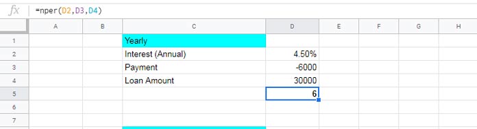
Let’s say you’re borrowing $30,000 at 4.5% annual interest, and you plan to pay $6,000 per year at the end of each period.
=NPER(4.5%, -6000, 30000)This returns the number of years required to repay the loan.
If the payment is made at the beginning of each year:
=NPER(4.5%, -6000, 30000, 0, 1)The fourth argument is FV (set to 0 since you’re fully paying off the loan), and the fifth argument (1) means the payment is made at the beginning of the period.
Note: Payments are shown as negative values because they represent cash outflows.
Example 2: NPER for Quarterly Payments
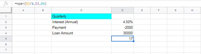
Suppose you want to make quarterly payments of $2,000 to repay a $30,000 loan at 4.5% annual interest.
Since the payment is quarterly, divide the annual rate by 4:
=NPER(4.5%/4,-2000,30000)This returns the number of quarterly payments needed to clear the loan.
Example 3: NPER for Monthly Payments
If you plan to pay monthly, divide the interest rate by 12. Here’s the structure:
=NPER(4.5%/12, -monthly_payment, loan_amount)You can plug in your own values as needed.
Calculate the Number of Periods to Reach an Investment Goal
Let’s say you want to save $20,000, and you deposit $500 at the beginning of each month into an account that earns 4.5% annual interest.
Here’s how to use the NPER function:
=NPER(4.5%/12, -500, 0, 20000, 1)This formula calculates the number of months required to reach your goal.
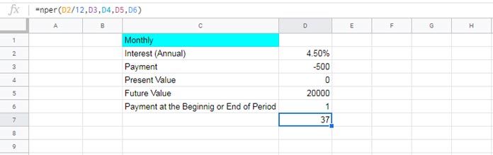
Result: You’ll need around 37 months to reach your $20,000 goal at that rate.
Tips for Using the NPER Function in Google Sheets
- In all examples, I’ve shown payments as negative values, representing cash outflows. The present value and future value are positive.
- Alternatively, you can use positive PMT values, but in that case, PV and FV must be negative.
Example:
=NPER(D2/12, D3, D4, D5, D6)
=NPER(H2/12, H3, H4, H5, H6)
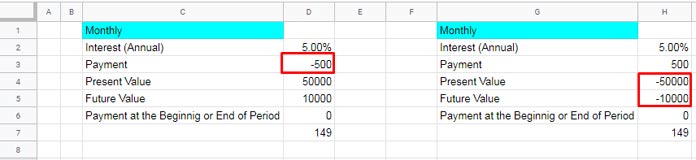
This ensures the signs align correctly and the formula returns expected results.
Final Thoughts
The NPER function in Google Sheets is an essential tool when planning loans or investments with regular payments. Whether you’re repaying a loan or saving toward a goal, this function helps you understand the timeline based on fixed interest and payment amounts.