Month Name as the Criterion in Date Column in Query Function in Google Sheets

Published on

Month Name is more reader-friendly. So it’s common to use month names like January, February … instead of month numbers like 1, 2… Here is a little tweak to use month name as the criterion in date column in Query in Google Sheets.

In Spreadsheets, month name as the criterion may not work as desired in formulas when using dates in formula ranges. Why so? Because month names are text strings. So you can’t compare it with the values in a date column.

Then how to use month name text as a criterion in a date column/field?

The solution is to convert month name string to month number and use that as the criterion.

This, other than the criterion part, I have well explained in one of my previous tutorials – Formula to Convert Month Name in Text to Month Number in Google Sheets.

In concise you can convert a month name string to its equivalent number as below.

Assume the cell A1 contains the month name January. The formula that converts this string to a number.

=month(A1&1)

But this won’t work in the same way in Google Sheets Query. There are two reasons.

  1. The count of month number in the Query is 0 to 11 not 1 to 12.
  2. The above formula extracts month number from a month name string. But the Month() scalar function is different in Query.

In the below examples, I am going to elaborate on how to use month name as the criterion in date column in Query in Google Sheets.

This GIF helps what I am talking about on this tutorial.

Month Name as the Criterion in Date Column in Query

How to Use Month Name as the Criterion in Date Column in Query Function

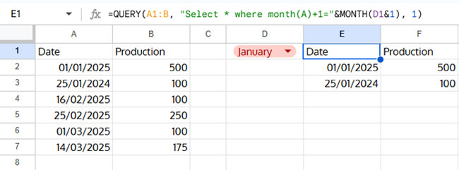
In Query, I want to use the criterion in cell D1 which is month name string. I have actually entered the month names as a list in Data validation to create that menu.

How?

Go to the menu Data and click on Data Validation. Choose criteria as “List of items” and paste the below list as it is in the given field (remove the double quotes).

“January,February,March,April,May,June,July,August,September,October,November,December”

This is for your convenience to quickly switch between the months. This cell, i.e. D1, you can use in the Query “Where” clause as the criterion in two ways.

You May Like: The Best Data Validation Examples in Google Sheets.

Query By Month Name in a Date Column (Field) Using Method # 1

This is the normal method, but little complicated.

If you know how to use the date as a criterion in Google Sheets Query, you can easily grasp it.

So before proceeding, please read my quick tutorial on the date criteria uses here – How to Use Date Criteria in Query Function in Google Sheets.

Hope you have gone thru’ that guide. Now see the formula that uses month name as the criterion in the date field in Google Sheets Query function.

=query(A1:B,"Select * where month(A) = month(date '"&text(DATE(2019,month(D1&1),1),"YYYY-MM-DD")&"')",1)

I have used the Month scalar function twice in this. The month() scalar function at the beginning of the “Where” clause tests the month in column A.

It has no issue in testing as column A contains dates. Then it matches that month number with the month number of the date in cell D1.

Since the value in cell D1 is text, I have used the Month worksheet function to convert that text to month number, i.e.;

=Month(D1&1)

You May Like: The ultimate guide on Google Sheets Date Functions.

Then with the help of the Date function, I have converted the returned month number to a date that falls in the corresponding month to the month name in that cell.

Then used the Month scalar function in Query to return the month number that Query can compare with the month number in column A.

There is one more simple way to use month name as the criterion in date column in Query. Here is that formula.

Query By Month Name in a Date Column (Field) Using Method # 2

This is very simple and my favorite choice. Here we only need to use the month scalar function once. First, let me share you the formula, then we can go to the explanation of that formula.

=query(A1:B,"Select * where month(A)+1 ="&month(D1&1)&"",1)

Yes! This is a small formula. Here is the detail.

The first month() scalar function directly checks the month number + 1 in column A with the month number in cell D1.

The +1 used to change the 0-11 month numbers in Query Month() scalar function to 1-12. Then only the month number matches with the Month worksheet function output 1-12.

In the first method, it’s not required because there I have compared the month number returned by the Month scalar function with the month number returned by another scalar function.

Here the comparison is between Month scalar function output and the Month date function output. The month date function returns 1 for January where as the month query scalar function returns 0 for January.

In this formula, you only need to take care of the double quotes used. That’s all about how to use month name as the criterion in date column in Query. Here are some additional resources to read.

Additional Reading:

  1. The Formula to Sort By Month Name in Google Sheets.
  2. Convert Numbers to Month Name in Google Sheets.
  3. Google Sheets Query: How to Convert Month in Number to Month Name in Text.
  4. Populate a Full Month’s Dates Based on a Drop-down in Google Sheets.
Prashanth KV
Prashanth KV
Your Trusted Google Sheets and Excel Guide Prashanth KV brings a wealth of experience in Google Sheets and Excel, cultivated through years of work with multinational corporations in Mumbai and Dubai. As a recognized Google Product Expert in Docs Editors, Prashanth shares his expertise through insightful blogging since 2012. Explore his blog for practical tips and guidance on maximizing your spreadsheet skills.

How to Extract Numbers from Text in Excel with Regex

You can use the REGEXEXTRACT or REGEXREPLACE functions to easily extract numbers from text...

Using OFFSET and MATCH Together in Google Sheets: Advanced Tips

One powerful and flexible way to look up values is by combining the OFFSET...

How to Use OFFSET and XMATCH Functions Together in Excel

We often use the OFFSET and XMATCH functions together to match a value in...

How to Calculate Maximum Drawdown in Excel and Google Sheets

You can use the following dynamic array formula to calculate maximum drawdown (MDD) in...

More like this

Using OFFSET and MATCH Together in Google Sheets: Advanced Tips

One powerful and flexible way to look up values is by combining the OFFSET...

Running Count with Structured References in Google Sheets

Running a count with structured references is achievable in Google Sheets tables using the...

Running Total with Structured Table References in Google Sheets

You can use two types of formulas to create a running total with structured...

LEAVE A REPLY

Please enter your comment!
Please enter your name here

This site uses Akismet to reduce spam. Learn how your comment data is processed.