From my perspective, we can insert three types of timestamps (or datetimes) into Google Sheets based on their behavior: dynamic, static, and conditional static.

Dynamic:

The auto-updating (dynamic) timestamp refreshes every time you edit your Sheet or when you reopen it. We use the built-in NOW() function for this.

Static:

The static datetime does not refresh or update when you modify your Sheet. We use a simple shortcut to insert it manually.

Conditional Static:

The third type is inserting a static conditional timestamp in Google Sheets.

In this method, we use an Apps Script to automatically insert a static datetime in one cell when we enter a value in another cell.

It updates only if that specific “trigger” cell changes — no other edits in the Sheet affect it.

Dynamic Datetime and the NOW Function

You can use the NOW() worksheet function in Google Sheets to insert a timestamp that updates on every edit.

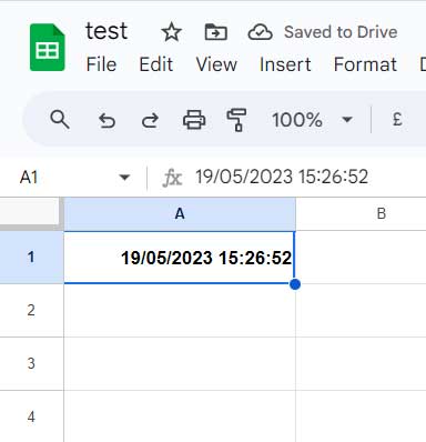
Just type =NOW() in cell A1 to insert the current date and time.

It will recalculate and refresh every time you make a change anywhere in your Sheet.

What else can you use it for?

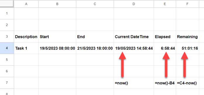
We can also use NOW() in logical tests. For example, if B4 and C4 store a task’s start and end times, you can calculate elapsed and remaining durations like this:

• =NOW()-B4 — Elapsed time
• =C4-NOW() — Remaining time

Real-Life Use: Dynamic Datetime Formula

You can find a practical example of using the NOW() function in my countdown timer tutorial.

Insert a Static Timestamp Using a Shortcut in Google Sheets

The best way to insert a static timestamp manually is by using keyboard shortcuts.

It depends on your OS:

• On Windows, press Ctrl + Alt + Shift + ;
• On Mac, press Command + Option + Shift + ;

(Note: In my testing on Mac, the shortcut didn’t work. Google’s documentation says, “Some shortcuts might not work for all languages or keyboards.”)

How to insert a static date and time in a cell:

• Select cell A1.
• Apply the appropriate shortcut.
• Check the formula bar — you’ll see the value is static (no formula inside).

Insert a Static Conditional Timestamp Using Apps Script

Earlier, Google Sheets allowed the creative use of LAMBDA functions to create conditional timestamps.

For example, you could use a formula like this in cell A1:

=LAMBDA(timestamp, IF(B1<>"", timestamp, IFERROR(1/0)))(now())

You could then copy it down the column to apply to multiple rows.

However, LAMBDA-based static timestamps aren’t reliable anymore.

So now, the best method is to Insert a static timestamp in Google Sheets using Apps Script.

Here’s a simple script for that:

function onEdit(e) {
  var sheet = e.source.getActiveSheet();
  var editedCell = e.range;

  // Define the specific range you want to monitor
  var watchColumn = 1; // Column A
  var timestampColumn = 2; // Column B
  var startRow = 2;
  var endRow = 10;

  // Only act if the edited cell is within A2:A10
  if (editedCell.getColumn() == watchColumn && editedCell.getRow() >= startRow && editedCell.getRow() <= endRow) {
    var cellValue = editedCell.getValue();
    var timeCell = sheet.getRange(editedCell.getRow(), timestampColumn);
    
    if (cellValue !== "") {
      timeCell.setValue(new Date());
    } else {
      timeCell.clearContent(); // Clear timestamp if the edited cell is cleared
    }
  }
}

This script is set to monitor the range A2:A10 and insert timestamps into B2:B10 when you enter values.

Modify for Other Ranges

You can easily adjust the script:

• To monitor A:A and insert timestamps in B:B, remove the startRow and endRow limits.
• To monitor C10:C50 and insert timestamps into D10:D50, change:
  • watchColumn = 3 (for column C)
  • timestampColumn = 4 (for column D)
  • startRow = 10
  • endRow = 50

How to Set It Up

1. Open your Google Sheets file.
2. Navigate to Extensions > Apps Script.
3. Delete any placeholder code and paste the above script.
4. Save the project (click the floppy disk icon).
5. Done! It works automatically — no need to manually run it.

This is how you can Insert a static timestamp in Google Sheets conditionally — automatically inserting a timestamp when a value is entered in a specific cell.