")
")


")


")

")
")
 in Excel & Google Sheets")


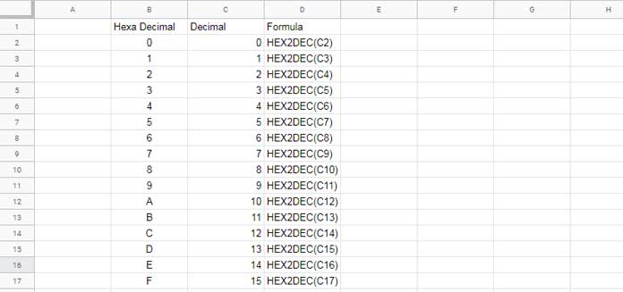
The HEX2DEC function in Google Sheets is categorized under Engineering functions. Its purpose is to convert a hexadecimal number, up to 10 characters long (40 bits), into its decimal equivalent.
What Is a 10-character Long, 40-bit Hexadecimal Number?
Let me explain. A hexadecimal (hex) system is a base-16 numbering system commonly used in computing. It uses 16 distinct digits: 0, 1, 2, 3, 4, 5, 6, 7, 8, 9, A, B, C, D, E, and F. In this system, each hex digit corresponds to a 4-bit binary value.
This means that the HEX2DEC function in Google Sheets can convert a hexadecimal number up to 40 bits (10 characters) to a decimal value.
In hexadecimal, the digits “0” to “9” represent values 0 to 9, while “A” to “F” (or “a” to “f”) represent values 10 to 15.
What Happens If You Exceed 10 Characters?
If you enter a hex number longer than 10 characters (exceeding 40 bits), the HEX2DEC function will return a #NUM! error. Hovering over the error message will show a tooltip like: “Function HEX2DEC parameter 1 is too long.”
Google Sheets HEX2DEC Function: Syntax and Arguments
Syntax:
HEX2DEC(signed_hexadecimal_number)Argument:
- signed_hexadecimal_number: This is the signed hexadecimal number you want to convert to decimal. The hex number cannot exceed 10 characters.
Details:
- The most significant bit of the signed_hexadecimal_number is the sign bit, while the remaining 39 bits indicate the magnitude of the number.
- Negative numbers are represented using two’s complement notation.
Examples of Using the HEX2DEC Function in Google Sheets
Example 1: Converting a Simple Hexadecimal Number
=HEX2DEC("5F")This formula returns 95. Here’s how it’s calculated:
- 5*16+15 (since “F” equals 15 in hexadecimal).
- HEX2DEC(“5”) x 16 + HEX2DEC(“F”)
Example 2: Converting a 3-digit Hexadecimal Number
=HEX2DEC("222")This formula returns 546. The breakdown is as follows:
-
=(2*16^2)+(2*16^1)+(2*16^0)
Example 3: Handling Leading Zeros in Hexadecimal
=HEX2DEC("000901")This formula returns 2305, calculated as:
=(9*16^2)+(0*16^1)+(1*16^0).
Example 4: Converting a Negative Hexadecimal Number
=HEX2DEC("FFFFFFFFFB")This formula returns -5. Here’s the breakdown:
The hexadecimal number “FFFFFFFFFB” is a 10-character signed hexadecimal number. Since it exceeds the 40-bit positive limit, it represents a negative number. In computing, negative numbers are stored using two’s complement format, which is a binary representation for negative values.
In expanded terms: =-16^9+(15*16^8)+(15*16^7)+(15*16^6)+(15*16^5)+(15*16^4)+(15*16^3)+(15*16^2)+(15*16)+11
Converting Unicode Values in Hexadecimal to Characters
You can use the CHAR function in Google Sheets to convert a decimal number into its corresponding Unicode character.
For instance, to insert a heart symbol in Google Sheets:
=CHAR(10084)However, Unicode tables often provide values in hexadecimal. The hex value for the heart symbol is 2764. If you only have this hexadecimal value, you can convert it to decimal using the HEX2DEC function:
=CHAR(HEX2DEC("2764"))This will also insert the ❤ symbol.
Conclusion
That’s everything you need to know about using the HEX2DEC function in Google Sheets. Whether you’re converting simple hexadecimal values or using two’s complement for negative numbers, this function is highly versatile. Enjoy exploring its capabilities!