With the help of flexible array formulas, you can automate overtime calculations in Google Sheets. However, you should use non-array (drag-down) formulas if you work on weekends and have a specific overtime rule for that.

The overtime calculation will be based on a daily threshold, such as 8 hours of regular time and 1 hour of lunchtime, with any hours worked beyond that threshold considered overtime.

You can customize the threshold value and lunch break hours. Additionally, you have the option to manually enable or disable lunch break subtraction, which is especially helpful for half-day work.

In this guide, you will learn one of the best overtime calculation formulas in Google Sheets. It’s flexible enough to meet your needs.

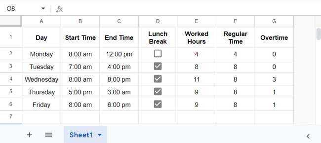
In our example, we have the start time in column B and the end time in column C. You can enable or disable the lunch break for specific employees by toggling the checkboxes in column D.

Let’s proceed with the step-by-step instructions.

Step 1: Streamline Worked Hours with a Formula

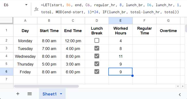
In cell E2, enter the following formula and drag the fill handle down as far as needed:

=LET(start, B2, end, C2, regular_hr, 8, lunch_br, D2, lunch_hr, 1, total, MOD(end-start, 1)*24, IF(lunch_br, total-lunch_hr, total))

Then apply Format > Number > Number.

In this formula, the lunch hour is specified as 1 hour. If you have a different lunch break duration, such as 30 minutes, replace 1 with 0.5 (30/60).

Another change is the regular working hours, which is 8 hours in the formula. You should change that based on your regular working hours in a day.

Formula Breakdown

The above formula lays the groundwork for automating overtime calculation in Google Sheets. The other calculations are straightforward. Let’s delve into it in detail.

The formula follows the LET function syntax:

LET(name1, value_expression1, [name2, …], [value_expression2, …], formula_expression)

It names value expressions and returns the result of the formula expression.

In the formula, start, end, regular_hr, lunch_br, and lunch_hr are self-explanatory. Regarding total, it is calculated as follows:

MOD(end-start, 1)*24 – calculates the worked hours.

Actually, (end-start)*24 would give the worked hours. However, it will provide a negative time difference if the end time spans past midnight.

MOD returns the remainder after dividing the time difference by 1. This ensures a positive time difference even if it spans past midnight.

For example, if the start time is 08:00 AM and the end time is 07:00 AM the next day, end-start would be -0.04 (if formatted as a number) and MOD(end-start, 1) would be 0.96 (if formatted as a number).

The time difference is the decimal portion representing the day, so we must multiply it by 24 to get the worked hours.

Here is the formula expression:

IF(lunch_br, total-lunch_hr, total)

If the tick box in column D is checked (lunch_br is TRUE), the formula subtracts the specified lunch_hr from the total; otherwise, it returns the total.

This checkbox unchecking ensures that the lunch hour is not subtracted from the worked hours of a person who worked half a day.

Step 2: Define Regular Time with a Formula

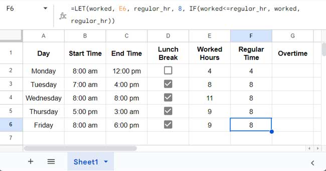
In cell F2, insert the following formula and drag it down as far as you need:

=LET(worked, E2, regular_hr, 8, IF(worked<=regular_hr, worked, regular_hr))

In this formula, you should replace 8 (regular_hr) with the stipulated regular working hours in your company. It should match the value (reular_hr) used in the formula in cell E2.

The IF function tests whether the worked hours are less than or equal to the regular working hours. If it evaluates to TRUE, it returns the worked hours; otherwise, it returns the regular hours.

Step 3: Automate Overtime Calculations

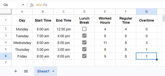
In cell G2, insert the following formula and drag it down:

=E2-F2

This formula will return the overtime hours by subtracting the regular hours from the total worked hours.

This method allows us to automate overtime calculations in Google Sheets.

Step 4: Handling Weekends and Holidays in Overtime Calculations

If you work on Saturday, Sunday, or any specific holiday, the overtime calculation may differ from the above. In such cases, all hours worked might be considered as overtime.

To accommodate this, you simply delete the regular time in column F from the corresponding rows.

That’s why I kept all the formulas as non-array formulas. If you don’t have entries for weekends and holidays, you can convert those three formulas into array formulas. Here they are:

=ArrayFormula(LET(start, B2:B6, end, C2:C6, regular_hr, 8, lunch_br, D2:D6, lunch_hr, 1, total, MOD(end-start, 1)*24, IF(lunch_br, total-lunch_hr, total))) // E2 formula
=ArrayFormula(LET(worked, E2:E6, regular_hr, 8, IF(worked<=regular_hr, worked, regular_hr))) // F2 formula
=ArrayFormula(E2:E6-F2:F6) // G2 formula

This concludes the process of automating overtime calculation in Google Sheets.

Resources

Here are some Google Sheets resources specifically for start-time and end-time calculations.

• Payroll Hours Calculation in Google Sheets
• Deducting Lunch Break Time From Total Hours In Google Sheets
• Combine Time In and Time Out into the Same Row in Google Sheets