


")


")

")
")
 in Excel & Google Sheets")


You may encounter a #REF! circular dependency error when attempting to place a column total in the first row of the same column using structured table references in Google Sheets. This error occurs because the formula references include the cell where the formula is placed. To resolve this, you can adjust the formula to exclude the first row from the calculation. For example, use a range that starts from the second row onward, like this:
=SUM(OFFSET(Table1[Column 1], 1, 0))This ensures the formula doesn’t reference its own cell, avoiding the circular dependency.
This will calculate the sum. Replace SUM with AVERAGE if you want to calculate the average instead.
In this formula, Table1 represents the table name, and Column 1 refers to the column you want to total.
Example of Displaying a Column Total in the First Row of a Structured Table
While it’s common to place the column total at the bottom of a table, there are times when you might want to keep the total visible without scrolling to the bottom. In this case, you can place the total in the first row of the table.
Let’s consider a table named Sales with two columns: Item and Amount.
To calculate the sum of the Amount column, enter the following formula in the first row of the same column, i.e., immediately below the column name:
=SUM(OFFSET(Sales[Amount], 1, 0))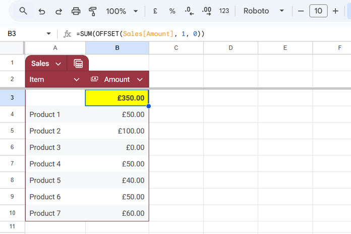
To calculate the average, replace SUM with AVERAGE:
=AVERAGE(OFFSET(Sales[Amount], 1, 0))If you want to exclude 0 from the average, use this formula instead:
=AVERAGEIF(OFFSET(Sales[Amount], 1, 0), ">0")We use the OFFSET function to shift the current row reference to avoid the circular dependency issue.
Unlike with regular ranges, when using structured references with OFFSET, you don’t need to specify the height argument. The function will offset by the number of rows and return the remaining values in the column.
Benefits of Using Structured Table References for the Column Total
Using structured table references for placing a column total in the first row—or in general—offers specific benefits.
In the example above, the actual range to total is B4:B10. You could place =SUM(B4:B10) in cell B3 to get the column total, but this approach won’t automatically capture newly added rows at the bottom of the table.
You might then think of using an open range, like =SUM(B4:B). While this works, it will include values below the table range, which can cause issues if you have unrelated data beneath the table, such as another table or other data not connected to the original table.
A structured table reference ensures that all rows within the table range are captured. The formula range will automatically expand as the table range grows.
Circular Dependency in Structured Table Reference in Google Sheets
When you insert a row by clicking the + button immediately below the first row containing the column total in a structured table, the formula in the first row and the cell below it may return a #REF! error.
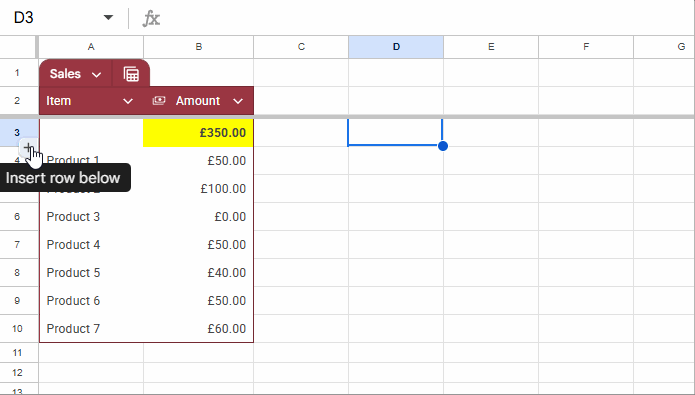
This occurs because the formula is automatically copied to the new row, creating a circular reference. To resolve this, simply delete the formula from the newly inserted row, and the column total will function correctly again.
Alternatively, you can right-click the row number and insert a new row without copying the formula.
Resources
Here are some resources related to structured tables in Google Sheets: