Essential Google Sheets Formulas for Your Budget Dashboard

If you’ve already downloaded my Free Household Budget Planner in Google Sheets, you know it comes with a clean dashboard and multiple tabs to track income, expenses, and savings. But have you ever wondered how the numbers and charts update automatically?

In this tutorial, I’ll walk you through the essential Google Sheets formulas that power the budget dashboard. You’ll see how functions like SUMIFS, ARRAYFORMULA, and QUERY connect your raw data to the summary view. Whether you want to customize the template, build your own version from scratch, or simply learn some practical Google Sheets tricks, this guide gives you a clear, behind-the-scenes look at how it all works.

Table of Contents

Introduction

The formulas in the free household budget planner template mainly depend on two sheets — Income and Expenses. Some formulas also use drop-downs in the dashboard to apply filters for month, all months, or year.

All tabs displayed in the Google Sheets budget template

If you already have my template, you can refer to the Expenses and Income tabs. Here’s a simplified version of the data:

Expenses table (named Expenses):

Date	Category	Description	Payment Mode	Amount
15/04/2024	🍽️ Food & Groceries	Groceries	G Pay	20000.00
16/05/2024	🍽️ Food & Groceries	Groceries	G Pay	25000.00
17/05/2024	💊 Health & Insurance	Medical Expense	Cash	20000.00
15/04/2025	🍽️ Food & Groceries	Groceries	Cash	7500.00

Income table (named Income):

Date	Source	Amount	Notes
20/04/2024	Advertising	45000.00
01/05/2024	Advertising	50000.00
10/01/2025	Advertising	0.00

We’ll use these sample structured tables in formulas across the Budget Overview, Annual Overview, and Helper sheets.

Calculating Annual Overview for the Budget Dashboard

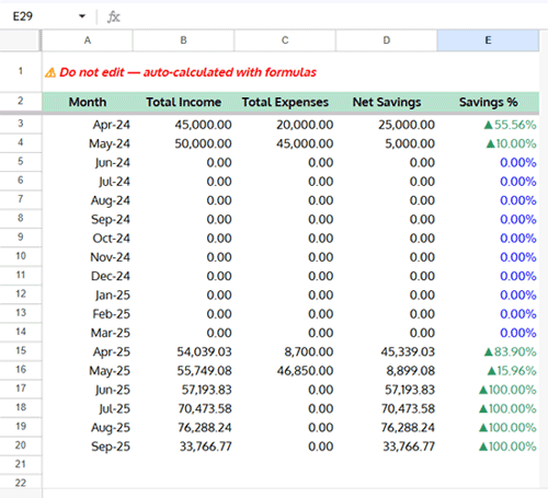
The Annual Overview tab contains 5 array formulas that create an annual summary. These don’t directly power the dashboard but will be used in the Helper tab to apply filters.

Annual Overview tab in the Household Budget Planner Google Sheets showing monthly income, expenses, savings, and savings percentage

1. Generate a Sequence of Months Based on Transaction Dates

Formula in A2:

=ArrayFormula(LET(
  dt, VSTACK(Income[Date], Expenses[Date]), 
  m, 
    EDATE(
      EOMONTH(MIN(dt), -2)+1, 
      SEQUENCE(DATEDIF(EOMONTH(MIN(dt),-1)+1, EOMONTH(MAX(dt), -1)+1 , "M")+1)
    ), 
  VSTACK("Month", m)
))

Explanation:

We used the EDATE function together with SEQUENCE to generate a continuous series of months, starting from the first transaction date and ending at the last transaction date. Here’s how the formula works step by step:

dt → Combines all transaction dates from both Income and Expenses into a single list.
MIN(dt) and MAX(dt) → Identify the earliest and latest transaction dates, so we know the full time span of your budget data.
EOMONTH(MIN(dt), -2)+1 → Finds the first month start one month before your earliest transaction. This ensures the timeline always begins neatly at the start of a month.
DATEDIF(…,“M”)+1 → Counts how many whole months exist between the earliest and latest transactions.
SEQUENCE(…) → Generates a list of numbers (1, 2, 3, …) equal to the number of months in that range.
EDATE(…) → Converts those numbers into actual month-start dates, giving us a clean timeline.
VSTACK(“Month”, m) → Adds a header and stacks all the month values underneath.

You get a clean, auto-generated list of months covering your entire budgeting period — no need to enter them manually.

2. Summarize Income by Month

Formula in B2:

=VSTACK("Total Income", ARRAYFORMULA(IF(A3:A="",,SUMIF(EOMONTH(Income[Date], -1)+1, A3:A, Income[Amount]))))

Explanation:

We used the SUMIF function to calculate total income for each month by matching dates from the Income table to the month list in column A. Here’s how the formula works:

EOMONTH(Income[Date], -1)+1 → converts each income date into the first day of its month (so all dates in the same month match consistently).
SUMIF(…, A3:A, Income[Amount]) → sums up the income amounts for each month listed in column A.
ARRAYFORMULA(…) → applies this logic across the entire column, so all months are filled automatically.
VSTACK(“Total Income”, …) → adds a header on top of the results.

Each month in column A now has its corresponding total income displayed in column B.

3. Summarize Expenses by Month

Formula in C2:

=VSTACK("Total Expenses", ARRAYFORMULA(IF(A3:A="",,SUMIF(EOMONTH(Expenses[Date], -1)+1, A3:A, Expenses[Amount]))))

Same logic as income, but using the Expenses table.

4. Calculate Net Savings

Formula in D2:

=VSTACK("Net Savings", ARRAYFORMULA(IF(A3:A="",,B3:B-C3:C)))

Subtracts expenses from income month by month.

5. Calculate Net Savings Percentage

Formula in E2:

=ArrayFormula(VSTACK("Savings %", IF(A3:A="",,(IFERROR(D3:D/B3:B, 0)))))

Divides net savings by income to calculate savings % per month.

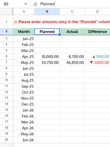
Calculating Budget Overview

The Budget Overview tab compares your planned budget vs. actual spending.

Budget Overview sheet in Google Sheets showing Planned vs Actual expenses and Difference column

Generate 10 Years of Months (A2)

=VSTACK("Month", ARRAYFORMULA(EDATE(DATE(2024, 12, 1), SEQUENCE(12*10))))

Produces months from Jan-2025 to Dec-2034 (120 months). Column formatted as MMM-YY.

This ensures the template supports many years ahead, so you can plan long-term budgets without manually updating the month list.

Enter Planned Monthly Budget in Column B

Formula in `C2`: Actual Expenses

=ArrayFormula(VSTACK("Actual", LET(xl, XLOOKUP(A3:A, 'Annual Overview'!A3:A, 'Annual Overview'!C3:C,), IF(xl=0,,xl))))

It pulls the actual monthly expenses from the Annual Overview tab, matching the months listed in column A.

Formula in `D2`: Difference

=ArrayFormula(VSTACK("Difference", IF((B3:B<>"")+(C3:C<>""), B3:B-C3:C,)))

It calculates the difference between your planned and actual expenses, so you can quickly see whether your spending is within budget or over.

Applying Filters in the Helper Tab

The Helper sheet filters data based on two dashboard drop-downs:

C1: Year filter
D1: Month filter (with extra option "All")

Interactive drop-downs for year and month selection in Google Sheets budget tracker

1. Filter Annual Overview Data

Formula in B2:

=IFNA(
  VSTACK('Annual Overview'!A2:E2, 
    FILTER(
      'Annual Overview'!A3:E, 
      ISBETWEEN(
        'Annual Overview'!A3:A, 
         DATE(Dashboard!C1, IF(Dashboard!D1="All", 1, MONTH(Dashboard!D1&1)), 1), 
         DATE(Dashboard!C1, IF(Dashboard!D1="All", 12, MONTH(Dashboard!D1&1)), 1)
      )
    )
  )
)

Helper tab in Household Budget Planner Google Sheets showing backend formulas for dashboard support

What this formula does:

It filters the Annual Overview tab for the year and month selected in the dashboard drop-downs, then displays the results with headers.

For example, if the year is set to 2025 and the month to May, the formula calculates the date range from May-01 to May-01, meaning only the transactions from May 2025 are returned. On the other hand, if the year is 2025 and the month is set to All, the range becomes Jan-01 to Dec-01, so the entire year’s transactions are included.

Explanation:

VSTACK → combines headers with filtered rows.
FILTER('Annual Overview'!A3:E, condition) → pulls only rows where condition is TRUE.
ISBETWEEN('Annual Overview'!A3:A, startDate, endDate) → checks if each row’s month start date falls between the chosen start and end dates.
Start Date = DATE(Dashboard!C1, IF(Dashboard!D1="All", 1, MONTH(Dashboard!D1&1)), 1) → If month = “All”, start is Jan-01 of the chosen year. Otherwise it’s the selected month start.
End Date = DATE(Dashboard!C1, IF(Dashboard!D1="All", 12, MONTH(Dashboard!D1&1)), 1) → If “All”, end is Dec-01. Otherwise it’s the same month start.

2. Expense by Category

Formula in H3:

=IFERROR(VSTACK(HSTACK("Category", "Expense"), 
  QUERY(
    FILTER(
      HSTACK(Expenses[Category], Expenses[Amount]), 
      ISBETWEEN(
        Expenses[Date], 
        DATE(Dashboard!C1, IF(Dashboard!D1="All", 1, MONTH(Dashboard!D1&1)), 1), 
        DATE(Dashboard!C1, IF(Dashboard!D1="All", 12, MONTH(Dashboard!D1&1)), 1)
      )
     ), "SELECT Col1, SUM(Col2) WHERE Col1 IS NOT NULL GROUP BY Col1 LABEL SUM(Col2)''")
))

Filters expenses by selected period, then groups them by category using QUERY.

3. Filter Budget Overview

In cells K3, L3, M3:

K3: =IFNA({B3:B})
L3: =VSTACK("Planned Expn.", ARRAYFORMULA(XLOOKUP(K4:K, 'Budget Overview'!A3:A, 'Budget Overview'!B3:B,)))
M3: =VSTACK("Actual Expn.", ARRAYFORMULA(XLOOKUP(K4:K, 'Budget Overview'!A3:A, 'Budget Overview'!C3:C,)))

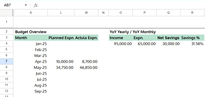
Google Sheets budget overview filtered by year and month with YoY income and expense comparison

This pulls planned and actual expenses side-by-side for the filtered months.

4. Compare Current vs. Previous Periods

Formulas in O4:R4:

O4 (Previous Income):

=SUMIF(
  ARRAYFORMULA(
    ISBETWEEN(
      EOMONTH(Income[Date], -1)+1,  
      DATE(Dashboard!C1-1, IF(Dashboard!D1="All", 1, MONTH(Dashboard!D1&1)), 1),  
      DATE(Dashboard!C1-1, IF(Dashboard!D1="All", 12, MONTH(Dashboard!D1&1)), 1)  
    )
  ), TRUE, Income[Amount]
)

P4 (Previous Expenses):

=SUMIF(
  ARRAYFORMULA(
    ISBETWEEN(
      EOMONTH(Expenses[Date], -1)+1,  
      DATE(Dashboard!C1-1, IF(Dashboard!D1="All", 1, MONTH(Dashboard!D1&1)), 1),  
      DATE(Dashboard!C1-1, IF(Dashboard!D1="All", 12, MONTH(Dashboard!D1&1)), 1)  
    )
  ), TRUE, Expenses[Amount]
)

Q4 (Previous Net Savings):

=O4-P4

R4 (Previous Savings %):

=IFERROR(Q4/O4)

What these formulas do:

These formulas compare the selected year and month in the dashboard with the same period in the previous year. For example, if the dashboard filter is set to May 2025, the formulas return totals for May 2024. If the filter is set to All for 2025, the formulas return totals for the entire year 2024.

Explanation:

The ISBETWEEN function checks whether each transaction falls within the same date range, but shifted back by one year.
SUMIF then totals the matching income and expense amounts.
Subtracting expenses (P4) from income (O4) gives net savings (Q4).
Dividing net savings by income calculates the savings percentage (R4).

Conclusion

We’ve now seen all the Google Sheets formulas powering the free household budget planner dashboard. From generating month sequences to filtering data dynamically, these formulas make it possible to track income, expenses, and savings in an automated way.

The Helper tab provides clean, filtered outputs that the dashboard charts and metrics use — so everything updates automatically when you change the drop-downs.

With these formulas, you can customize your Google Sheets budget dashboard, expand it to multiple years, or simply learn new tricks to manage your finances better.

If you’d like to try these formulas in action, grab the free template and start customizing your own budget dashboard today.

Get Your Free Template