If you’re familiar with Excel, you may notice the absence of the formula auditing feature, which allows you to trace precedents and dependents, in Google Sheets.

In Excel, you can find the formula auditing tools on the Formulas tab, within the Formula Auditing group. Keyboard shortcuts such as Alt + T + U + T (trace precedents), Alt + T + U + D (trace dependents), and Alt + T + U + A (remove arrows) make this process efficient. I extensively relied on these shortcuts.

Unfortunately, this feature is missing in Google Sheets. The only available options are workarounds, and they do not come close to Excel’s formula auditing capabilities.

There are workarounds both with and without using add-ons. If you prefer not to use add-ons or are dissatisfied with them, this tutorial might assist you to some extent in performing formula auditing in Google Sheets.

The Purpose of Formula Auditing in Spreadsheets

Trace Precedents is employed to identify the cells or arrays used in a formula, ensuring the correct references are applied.

For example, when using the SUM function for a total at the bottom of a column, trace precedents visually highlights the range utilized in that formula.

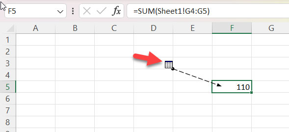
Excel indicates arrays or ranges with a border, dots on cells, and connecting arrows to visually identify precedents. If the reference is on a different sheet, a small icon appears, allowing you to double-click on its bottom-right corner to open the Go To dialog box.

The trace dependents formula auditing feature serves to verify whether a cell or array is part of any formula. This is helpful before deleting a value in a cell or array or before moving or deleting an array, featuring the same visual identification cues.

Regrettably, Google Sheets lacks the aforementioned Trace Precedents and Trace Dependents formula auditing tools. There is no genuine alternative to Excel Formula Auditing in Google Sheets. Presented here are workarounds without relying on any add-ons.

How to Do Formula Auditing in Google Sheets

Before delving into the topic, consider this crucial point: Embrace Array Formulas whenever possible. Begin by using Array Formulas—formulas that extend from one cell to a range—whenever applicable. You can convert most formulas into expanding ones using ARRAYFORMULA or LAMBDA helper functions. This approach often simplifies formula structures and reduces the need for extensive auditing.

Also, use closed ranges, such as A1:Z1000, instead of open ranges like A:Z or A1:Z, in formulas if you want the trace dependents workaround approaches to work correctly.

Now, revisiting formula auditing in Google Sheets, we’ll explore four workarounds for trace precedents (two) and trace dependents (two) formula auditing.

Precedents:

1. Leveraging the F2 cell edit feature (F2 in Windows and Shift + Enter/Return on Mac)
2. Using the Go to Range command.

Dependents:

1. Utilizing a combination of the Show Formula (Ctrl+`) feature and the Find (Ctrl + F in Windows and Command + F in Mac) command.
2. Applying a regular expression match using the Find and Replace (Ctrl + H in Windows and Command + Shift + H in Mac) command.

Trace Precedents Formula Auditing in Google Sheets

Alternative to Trace Precedents in Google Sheets (Excel alternative):

Follow these steps:

1. Navigate to the cell containing the formula for which you want to find the precedents (audit).
2. Press the F2 keyboard shortcut in Google Sheets on Windows, or use Shift + Enter/Return on Mac. Alternatively, you can double-click on the cell. The cells connected to the formula will be highlighted with colored dots.
3. Move the cursor pointer to the left using the left arrow key on your keyboard. It will highlight the cell or range used in the formula one by one.

This serves as an alternative solution to Excel Formula Auditing in Google Sheets for Trace Precedents.

Drawback:

If the formula uses references to another sheet in the same Google Sheets, this method won’t yield the result.

How to go to the range used in a formula:

In Excel, as mentioned at the beginning, we can double-click on a small icon to go to the range of the formula.

Here, instead, you can follow one of the below methods:

• Copy the reference from the formula. Then go to the Name Box using Ctrl + J in Windows and Command + J in Mac. Paste the reference and hit enter. The Name Box is a small box at the left of the formula bar.
• Alternatively, you can click on Help > Search the menus > Go to range and paste the reference, then hit enter or click on the > button.

Trace Dependents Formula Auditing in Google Sheets

Alternative to Trace Dependents in Google Sheets (Excel alternative):

When it comes to Trace Dependents, you may keenly feel the absence of the Excel formula auditing feature. Even the workaround may not fully meet our requirements here.

Here are the best Trace Dependents workarounds in Google Sheets.

Using Show Formula and Find Command

Use this when you want to search for a specific cell or range used in a formula, such as A5 or B10:C20.

In the following example, I want to test whether cell B5 has any dependents. Let’s see how to find that.

Steps:

1. To do this, first, use the shortcut key Ctrl + ` (Both in Windows and Mac) or click on View > Show > Formulae.
2. Then use Ctrl + F in Windows and Command + F in Mac to open the Find dialog box.
3. Enter the cell or range reference and hit enter. It will highlight the formulas that use the exact cell or range reference.

Drawbacks:

There are two potential drawbacks to this approach.

• It can only match the exact range or cell. If you want to find any formula dependent on cell B5 while the formula uses B1:B100, it won’t work.
• It applies to the sheet that you search, if the cell or range reference has any dependents in any other sheet, it won’t highlight them.

We will try to address these trace-dependent drawbacks in the next approach.

Using Find and Replace Command and Regular Expression Match

We can use the Find and Replace command as an alternative to solve the second drawback mentioned above.

1. Click on Edit > Find and Replace (Ctrl + H in Windows and Command + Shift + H in Mac) command. Here, there’s no need to enable the “View formulae” as mentioned earlier.
2. Enter the cell or range address, including the sheet name if any, in the Find field.
3. Leave the “Replace” field empty.
4. Other settings are as follows:
   • Search: All Sheets.
   • Check “Also search within formulae.”
5. Then click on “Find” to locate the dependent formula(s) within the current sheet or another sheet in that workbook.

But how do we trace dependents of a cell or cell range in Google Sheets that is part of a bigger cell range?

Here, you can use the following regular expression within the Find and Replace, for cell ranges that use row numbers in the range. It won’t support A1:C, A:D, etc., as they do not have row numbers on both ends, or either end. It will work with cell ranges such as A1:C1000, D6:F500, etc.

Regular Expression:

\b[A-Z](\d{1,5})\b

How do we use it?

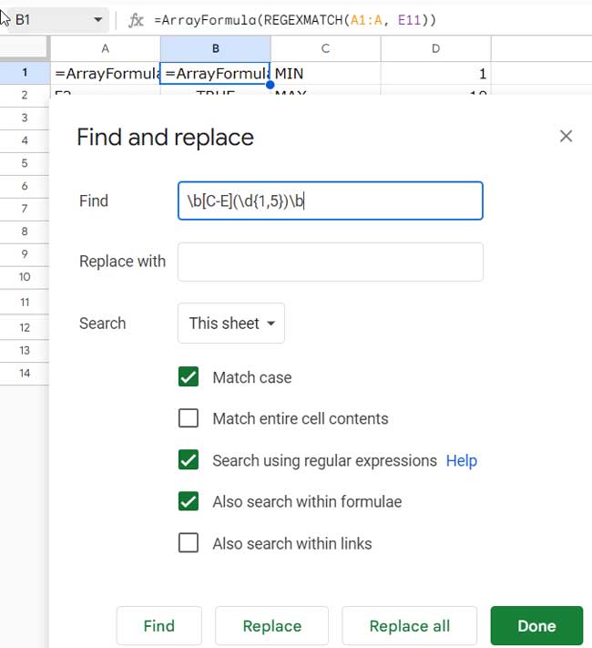
In the fourth step above, check “search using regular expressions” and select “This sheet” instead of “All sheets.” All other settings remain the same.

Example:

Assume you want to check whether cell E11 is part of any formula.

\b[C-E](\d{1,5})\b

Use this regular expression within Find and Replace, as detailed above, to find the dependent formula that uses cell references from columns C to E.

Note: Similar to Excel formula auditing, this method won’t locate the dependent if the starting and ending columns in the formula are outside of columns C to E (e.g., it won’t locate =SUM(A1:F100))

Drawbacks:

• This will match strings that contain cell references. For example, the above will match if any cell contains the string E11.
• Not useful to trace dependents in multiple sheets.
• It locates the dependents of whole columns, not specific cells or ranges. For example, if a formula uses any cells in column A or B, it will locate that formula if you specify [A-B].

Conclusion

I’ve presented several alternatives to Excel formula auditing in Google Sheets.

I hope this tutorial fulfills the requirements of tracing precedents and dependents for those who do not wish to use add-ons.

Certainly, Google Sheets add-ons can simplify tracing precedents and dependents. If you are comfortable, you can install them by clicking on the menu Extensions > Add-ons > Get add-ons from within your Google Sheets file.

If you aren’t comfortable giving permission to apps, then the workarounds are the only way for now.